
Introduction
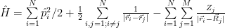
Last time we ended up with a simplified Hamiltonian:
and having the variational principle for help. It turns out that this simplified Hamiltonian is not simple enough. In this post I’ll expose one method that allows one to do calculations for quite complex quantum systems, the Hartree-Fock method. Because the subject is quite large, obviously I cannot cover it into detail in a blog post. Entire books were written about it, or the method is a large part of books treating for example computational chemistry, but even those might not cover some details, as computing the integrals for example, but more about that, later.
This post will be followed by one that will describe a Hartree-Fock program1 I implemented. I intend here to focus on theory and there to give more details about implementation.
Since I cannot give all the details here, I’ll point to links/articles with more info. Here is one for the start: A mathematical and computational review of Hartree-Fock SCF methods in Quantum Chemistry2 by Pablo Echenique, J. L. Alonso.
The Hartree term
The big problem with the Hamiltonian above comes from the second term. The other two can be written together as a sum of uni-particle Hamiltonian terms. Thanks to Born Oppenheimer approximation discussed last time, the potential of the nuclei is not time dependent, which would allow solving it relatively simple. The problem comes from the electron-electron interaction term. An approximation would be to consider each electron as interacting with an average potential given by all other electrons, as in mean field theory.
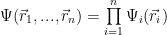
Let’s make some simplifying assumptions that are plain false and not that useful, but we’ll ‘fix’ them later. First, let’s assume that the electrons are non interacting, in the sense that instead of interacting with each other, they will generate together a mean field with which they interact. Then, let’s presume they have no spin. With those assumptions, we can describe individual electrons by wave functions, that is, each electron is described by a wave function and we can write the wave function for all electrons as a product of individual wave functions:
One gets for the j electron wave function the equation:

The first two terms are the kinetic energy term and the nuclear attraction potential energy term, respectively. The third one is the Hartree term. If one interprets the 

This equation has issues, for example it completely neglects electrons correlations. The assumption that the electrons are non interacting and they can described separately by wave functions is false. Even if we are trying to use a product of uni-electron wave functions we should take into account that electrons are not distinguishable. Electrons are fermions and they obey the Pauli exclusion principle.
Another issue is that the electron interacts with its own field. This could be solved by avoiding summing j in the last term, but then each electron will interact with a different field.
The Hartree operator is also called the Coulomb operator and the sum of the kinetic energy operator and the nuclear attraction potential energy operator, the core operator.
Some of the issues are solved by an additional exchange term that I’ll detail later.
Slater determinants
As mentioned above, the wave function 

It is easy to verify that the probability of having both electrons in the same point becomes zero.
The exchange term. Hartree-Fock equations.
One can derive the Hartree-Fock equations using variational calculus, minimizing the energy functional for a Slater determinant. I don’t want to give all details here, for details you could look into the review article I already mentioned or in Derivation of Hartree–Fock Theory3.
From now on I’ll use 


The exchange term is:
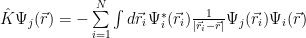
The minus sign is because of the anti-symmetry, the resulting operator being a non-local one. The Fock operator is:

The Hartree-Fock equations are:

I should mention here, just in case you noticed the featured image, that there is an implicit summation for spin which I did not detail. So now you know where the 2 comes from in the featured image: there are two electrons of opposed spin in the same orbital. The formula is for the restricted Hartree-Fock method which I’ll detail later.
The exchange term deals not only with the exchange, but cancels the self-interaction of the electron, too.
Now we have some equations that look familiar. They look like the eigenvalue problem, it looks like we have linear equations. It’s just the Schrödinger equation with the electron-electron interaction given by the Coulomb and exchange operators, right? The looks can be deceiving, the Fock operator depends on the eigenvectors, the equations are non linear! We have a set of coupled non-linear equations.
The method for solving it is by guessing some initial wave vectors for the solution, fit them into the Fock operator, solve the Hartree-Fock equations to get new wave vectors, replace the old ones into the Fock operator, solve again the equations, repeating the procedure until eigenvalues and/or eigenvectors do not change appreciably (some other more complex convergence criteria might be used, too), that is, the solutions converge. That’s why the method is also called the self consistent field method. It looks like first the electrons start in some orbitals that create a certain potential. The potential acts on the electrons that ‘adjust’ by moving into adjusted orbitals that generate another potential and so on, until the electrons end up in stable orbitals that do not change anymore under the influence of the potential.
Basis sets
You may try to solve the equations numerically, although they are not exactly easy to solve (they are integro-differential ones). There is a method that allows us to solve them algebraically. For that, we use the superposition principle to write the wave functions as a sum of projections onto basis states. In matrix representation, the wave functions are column vectors, with the projection values as elements (that is, 

So the wave function can be decomposed using a basis:

If the basis wave functions would be orthogonal, the equations would look the same, that is, like the regular eigenvalue problem, just that the wave functions would be replaced by column vectors and operators with matrices. In general, they do not need to be orthogonal, in which case the overlap matrix S – with matrix elements 
They used first Slater-type orbitals for the basis functions, they are still used for example for a single atom, but the difficulty of solving the integrals with different centers made the Gaussian orbitals a better choice. More precisely, they use linear combinations of Gaussians, like STO-nG, to approximate better a Slater-type orbital.
Currently the Hartree-Fock program1 I implemented uses STO-3G and STO-6G although is should be easy to extend to be able to use other basis sets as well. You may find out more about basis sets on Wikipedia. Here is a good start for Linear Combination of Atomic Orbitals. The source of the basis sets I used is here: EMSL Basis Sets Exchange4.
Roothaan Equations
In the closed shell case, all orbitals up to the ones in the valence shell are doubly occupied, that is, they are filled with two electrons of opposite spins. For such a case one can sum out the spins from Hartree-Fock equations (in matrix form), obtaining the Roothaan equations. They are already in the featured image, but here they are, again:

Keep in mind that the sums from the J and K operators now go over the occupied orbitals, not over the number of electrons.
Density Matrix
I don’t want to detail the operators in the equations, you may find details in the links I provided, but I thought that I should I least mention the Density Matrix. For example for the restricted Hartree-Fock method, the density matrix operator is:

The matrix element as seen in the implementation is:
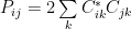
2 appears because of the two electrons occupying an orbital.
Pople-Nesbet Equations
I also thought that I should mention the unrestricted method. I implemented it in the program, but I don’t want to detail it much, either here or in the post describing the code. If interested, you can check out the links and the code1.
The Pople-Nesbet equations are:


They are obtained by eliminating the restriction of having two electrons occupy the same orbital, that is, each electron has its own orbital. This way one can deal with open shell atoms/molecules. Those equations are coupled, there is an additional term in the Fock operators that contains the density matrix for the other spin, that is, the ‘up’ equations also contain the density matrix for the ‘down’ electrons and viceversa. It should be obvious why, there is a coulomb interaction between ‘up’ and ‘down’ electrons, too.
Gaussian integrals
This subject is huge, I won’t say much about details here. Here are some very brief ideas:
Gaussians are used because the product of two Gaussians is also a Gaussian and the Gaussian functions and their Gaussian integrals occur a lot in physics, so they are quite studied. Since the Hartree-Fock method was developed, a lot of work was put into finding better methods of calculating those integrals. By the way, in the order of complexity they are: the overlap integrals, the kinetic integrals, the nuclear attraction integrals and the electron-electron integrals, the later being the hardest to solve. You might also need to calculate the dipole moment (or even multipole-moment) integrals, for example if you want to compute the spectrum. Electron-electron integrals calculations need a lot of computing time and memory. For a complex molecule one might need to save them on disk or simply discard them and recalculate them again at the next iteration.
There are several methods, I just picked one for the program that seemed easier to implement but also fast enough. A naive approach ends up with calculating the same integral many times, with a lot of loops into loops into loops … you should get the picture by now … with binomial coefficients and so on, which is quite slow. They obtained better results by hitting the integrals with derivatives and other mathematical tricks obtaining recurrence relations which one can use to calculate them. I won’t enter into details, but I’ll give some links to some pdfs that might help. First, a general one that contains an entire chapter about molecular integral evaluation, although I don’t think it would be enough for writing a program able to calculate them, but it should give you an idea: Advanced Computational Chemistry5. You may find more things in there, about the variational principle, basis sets, Hartree-Fock, and so on. Here is another one, just about molecular intergrals: Fundamentals of Molecular Integrals Evaluation6. That should suffice for now, I’ll give more links when I’ll describe the Hartree-Fock program1.
For the case of calculating the electron-electron repulsion integrals, using integrals permutation symmetries is mandatory, there are a lot of them and they are quite expensive to calculate. Using those symmetries allows you to calculate approximately 8 times less.
By the way, you’ll meet in those papers not only the Dirac notation but also a notation used by chemists, which even makes sense if you think in terms of density. It’s not a big deal:

For a contraction they use ![[ij|kl]](https://s0.wp.com/latex.php?latex=%5Bij%7Ckl%5D&bg=ffffff&fg=000&s=0&c=20201002)
What can be calculated
It should be obvious by now that the method allows calculating the ground state and the ground state energy. Since one can also calculate it not only for the molecule, but for the individual atoms that are in that molecule, one can get the binding energy. One can also calculate the dissociation energy. Since the method does not force you to have a neutral atom or molecule, you may put in there either more electrons to get negative ions, or less to have positive ions. This way you can calculate electron affinity and ionization energy.
You may want to calculate excitation energy. You could change the program to complete the orbitals accordingly (the variational principle works for excited states, too). I did not implement that, yet, although it’s not a very big deal.
As a shortcut, you could use Koopmans’ theorem.
A lot more can be done, but quite a bit of additional work would be involved, from computing the molecular structure to computing the electronic spectrum or the vibrational-rotational one. If you want to go there, you might want to implement a Post Hartree-Fock method to get better results.
Conclusions
I presented briefly some theory about the Hartree-Fock method, next time I’ll describe the Hartree-Fock program1. This is a blog entry, not a lecture or a book, so I couldn’t cover it more. There might be quite a bit of mistakes or unclear things in the text, if you notice them, please let me know and I’ll correct them.
- A Hartree-Fock program The project on GitHub. ↩ ↩ ↩ ↩ ↩
- A mathematical and computational review of Hartree-Fock SCF methods in Quantum Chemistry Pablo Echenique, J. L. Alonso ↩
- Derivation of Hartree–Fock Theory Arvi Rauk ↩
- EMSL Basis Sets Exchange Source of the basis sets used in the program. ↩
- Advanced Computational Chemistry Pekka Manninen ↩
- Fundamentals of Molecular Integrals Evaluation Justin T. Fermann and Edward F. Valeev ↩
