
Introduction
Newton is considered as being the one that started the modern physics, so something related with his work seems appropriate to start this blog.
Besides, I had an old program simulating a solar system that I wrote quite a while ago. I wrote the program with the old OpenGL fixed pipeline and leapfrog integration, on Linux, with glfw and now I decided to rewrite it using shaders. I considered it a good opportunity to refresh my memory about OpenGL so maybe I got a little carried away and added too much for the purpose of this blog, but about that, later.
Despite the simplicity of the subject this is a good start for various topics, like numerical methods for solving complicated differential equations or the field of molecular dynamics and before going into more complicated matters for those, this could be a good introduction, so here it is.
The subject is a very simple molecular dynamics program that simulates a solar system using Newtonian mechanics and the Newtonian law of universal gravitation, that is, an N-Body simulator (more specifically, a direct N-body simulation).
Before you run away, here is a video of the end product, maybe you decide to read on:
The Physics
One does not need to know a lot of physics for dealing with such a subject. Oddly enough, even simulations of large scale on supercomputers do not go way much beyond this (for direct methods, with the loss of accuracy they actually can go down to O(N log N) or better, see the links provided for details), they still use Newtonian gravity and a simple integration method like the one used here. The reason is that for the purpose the Newtonian mechanics is good enough. The simulated objects do not travel at large enough speeds and they are not subjected to gravitational fields that change things so much to matter. The numerical errors are usually larger than the relativistic effects differences.
You need to know only Newtonian mechanics and Newtonian gravity and that’s about it. The emphasis is on 


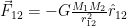
So, the force acting on the body i is:

This is our plain old 

Since we are not really interested in the forces, but in the change of position, we actually need the accelerations. It is quite straightforward to implement, so without more stories, here is the code that calculates the acceleration:
1 2 3 4 5 6 7 8 9 10 11 12 13 14 15 16 17 18 19 20 21 22 | inline void ComputationThread::CalculateAcceleration(BodyList::iterator& it, BodyList& Bodies) { static const double EPS2 = EPS*EPS; Vector3D<double> r21; double length; it->m_PrevAcceleration = it->m_Acceleration; it->m_Acceleration = Vector3D<double>(0., 0., 0.); for (auto cit = Bodies.begin(); cit != Bodies.end(); ++cit) { if (cit == it) continue; r21 = cit->m_Position - it->m_Position; length = r21.Length(); it->m_Acceleration += r21 * cit->m_Mass / ((length*length + EPS2) * length); } it->m_Acceleration *= G; } |
The code should be easy to understand, r21 is the 

Molecular dynamics
Molecular dynamics is basically this: you have a bunch of ‘particles’ in a physical system, you know the initial state which is given by all the particle positions and momenta, or in the simple cases when the mass of particles stays unchanged as known in the beginning, their velocities. You want to know the evolution of the system over time. For that you calculate all particle interactions – and here it can be quite messy, too, you might need to deal with quantum mechanical interactions – and then using them you want to change the particles positions and velocities using the equations of motion so you obtain the state of the system after an instant of time. Do that a lot of times and you can extract a lot of information about the system. Hopefully I’ll get back to molecular dynamics on this blog so I won’t insist much here on this subject. Finally, here is the code that implements it:
1 2 3 4 5 6 7 8 9 10 11 12 13 14 15 16 17 18 19 20 21 22 23 24 25 26 27 28 29 30 31 32 33 34 | void ComputationThread::Compute() { unsigned int local_nrsteps; const double timestep = m_timestep; const double timestep2 = timestep*timestep; BodyList m_Bodies; GetBodies(m_Bodies); for (auto it = m_Bodies.begin(); it != m_Bodies.end(); ++it) CalculateAcceleration(it, m_Bodies); for (;;) { local_nrsteps = nrsteps; // do computations for (unsigned int i = 0; i < local_nrsteps; ++i) VelocityVerletStep(m_Bodies, timestep, timestep2); CalculateRotations(m_Bodies, local_nrsteps*timestep); // give result to the main thread SetBodies(m_Bodies); // is signaled to kill? also waits for a signal to do more work { std::unique_lock<std::mutex> lock(mtx); cv.wait(lock, [this] { return an_event > 0; }); if (an_event > 1) break; an_event = 0; } } } |
After the first initialization phase, the for(;;) loop simply does the calculations using Velocity Verlet, advancing several time steps (as configured by the main thread) before returning a result to the main thread and waiting either for a request for more data or for exit.
Simplifications
In this case, the gravitational force range is infinite and there is no screening possible so one has to consider the interaction of a ‘particle’ with all the others. In other cases it might be simpler, when there is screening and/or the range of the interaction is limited one could consider only the neighbors of a ‘particle’ for interactions, using neighbors lists that are updated once in a while after performing many time steps in the simulation. That does not mean one cannot simplify/increase the speed of gravity simulations. In some cases one could ignore interactions with bodies that are far away and have no considerable mass, depending on what the purpose is. In other cases, a bunch of ‘particles’ can be considered a single body and a center of the mass approximation could be used or perhaps some first terms from a multipole expansion. Depending on the place they are one could use different time steps. For details and more methods, please visit the wikipedia links provided above. Anyway, for this simulator I chose to calculate all interactions between simulated bodies, although there are some simplifying assumptions.
One of them is ignoring the influence of the objects not simulated, obviously. I did not add all the moons and asteroids and comets… and the other stars in the Universe except the Sun. To see why it does not matter that much one could try to calculate the gravitational influence on him from his favorite star, the one that his astrologer claims to influence his life. It is instructive to compare it with the tiny gravitational influence from some nearby building or tree. Also one could notice that the Universe does not really care much about the direction in space so if the star that influences your life pulls you towards it, there might be another star in the other direction that cancels the pull (see below the comment about spherical symmetry for more). But let’s suppose there isn’t. Don’t forget that the tiny pull on you is also on the Earth, so you and the Earth are both falling towards that star with the same acceleration (and the star is falling towards you, but you should not care about that, it’s not going to hit you soon, to care that much, and besides it’s a matter of perspective, anyway). How did the astrologer say the star is influencing you and only you and some other chosen ones? You and the Earth and everybody else are free falling towards that star and the effect that could affect you is way tinier than even the tiny force you calculated suggests.
I’m sorry about the rant on astrology but it’s incredible how many still believe that (and other quite similar) bullshit.
Another assumption made is that the bodies are spheres with the mass distributed in a spherically symmetrical manner. Using Gauss theorem one can check that for a spherical shell with spherical symmetry of the mass distribution the gravitational field outside is as if all the mass is in the center of the sphere. Also the field inside is zero, a fact that was missed by a lot of science fiction stories about a hollow Earth or Moon or whatever hollow planet. From that it’s easy to see how a sphere with spherically symmetric mass distribution has the same gravitational effect as if its whole mass is in its center (again, outside of the sphere). To see why this is a quite good assumption one can calculate the field from a ‘dumbbell’ composed of two point masses placed at a small distance compared with the distances where they act. Or, more generally, one could consider the multipole expansion.
Numerical method
The numerical method used is Velocity Verlet but before going to that, I want to describe an easier method that is both easier to understand and implement: the Euler method. Consider the derivative definition:
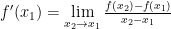
You can already see that in our case velocity and acceleration play the role of the generic f and the variable is time. More often than not, you have no chance of analytically solving the problem (with is also the case for the N-Body problem, except when N=2 or with restrictions, 3). You may have a chance to solve it numerically, with the computer. For that you have to forget the 

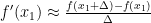
Arranging it a little you get the Euler method: 


Geometrically it is easy to see that while the derivative is given by the slope of the tangent to the function in the calculation point, the Euler method uses the chord instead (the line segment between the 

I had an old program where I implemented the Leapfrog method, but for this post I decided to use the Verlet integration. By now I think I’ve given enough information (less in the text, more in the links) for understanding Velocity Verlet. I mentioned the difference method and with the addition of the story about the chord versus tangent one can see how the central difference is better. Applied on the acceleration one gets the Verlet integration without velocities. Now with a little help from the Leapfrog method one should get the Velocity Verlet, too. The details are in the links. By the way, hopefully you notice the similarities with 

1 2 3 4 5 6 7 8 9 10 11 12 | inline void ComputationThread::VelocityVerletStep(BodyList& Bodies, double timestep, double timestep2) { for (auto &body : Bodies) body.m_Position += body.m_Velocity * timestep + 0.5 * body.m_Acceleration * timestep2; for (auto it = Bodies.begin();it != Bodies.end(); ++it) { CalculateAcceleration(it, Bodies); it->m_Velocity += (it->m_Acceleration + it->m_PrevAcceleration) * timestep * 0.5; } } |
It should be very easy to understand, timestep2 is the square of the timestep (just an optimization to avoid recalculating it in several places repeatedly), the others should be self describing. There are three parts:
- Update the position.
- Calculate the acceleration at the new position. Because the position for the current time is needed for all bodies, the previous part is executed in a loop for all bodies before reaching this part.
- Use the accelerations at the previous and new positions to calculate the velocity at the new position.
The Code
If you did not get the code1 by now, you probably should get it. I put it on GitHub, here. From the pieces of code presented above, you probably figured out the the molecular dynamics code is in a separate thread implemented in a class named ComputationThread. There is no much to it besides what is already presented, except some things related with thread starting/synchronization/data accessing. Here is the method that calculates the rotations, for the others I’ll let you look into the code:
1 2 3 4 5 6 7 8 9 10 | inline void ComputationThread::CalculateRotations(BodyList& Bodies, double timestep) { for (auto &body : Bodies) { double angular_speed = TWO_M_PI / body.rotationPeriod; body.rotation += angular_speed * timestep; if (body.rotation >= TWO_M_PI) body.rotation -= TWO_M_PI; else if (body.rotation < 0) body.rotation += TWO_M_PI; } } |
There is not much to this method, hopefully you did not expect one that gives precession, nutation, that is, a full rigid body treatment. The first two lines in the for loop are pretty straightforward, they implement the simple rotation around the axis, the other two are there just to keep the value in the ![[0,2\pi]](https://s0.wp.com/latex.php?latex=%5B0%2C2%5Cpi%5D&bg=ffffff&fg=000&s=0&c=20201002)
Now, here is a short description of the classes (also in the README file):
First, the classes generated by the MFC Application Wizard:
CAboutDlg – What the name says, I don’t think it needs more explanation.
CMainFrame – Implements the main frame. Besides what was generated (adjusted to fit the application needs), I added code to deal with menu entries, some message routing to the view and that’s about it. CMainFrame::OnFileOpen deals with opening a configuration xml file for the solar system. CMainFrame::OnViewFullscreen besides switching the full screen, it also hides the mfc toolbar that allows closing the full screen.
CSolarSystemApp – Implements the application object. Not much change there, besides setting a path for registry settings, setting the main window title and loading the ole libs (needed for MS xml parser)
CSolarSystemDoc – Contains and manages the computation thread (m_Thread) and the solar system data (m_SolarSystem). Most of the code deals with loading the xml file, using MS XML parser. There is also some code that deals with the computation thread.
CSolarSystemView – The view. Deals with OpenGL setup, displaying the scene (look into the Setup methods) and also with the keyboard and mouse message handling. CSolarSystemView::OnDraw is the drawing method. CSolarSystemView::RenderScene does the actual drawing, CSolarSystemView::RenderShadowScene is a quite simplified version of the previous, dealing only with shadows, CSolarSystemView::RenderSkybox draws the skybox. CSolarSystemView::MoonHack is a ‘moon hack’ that allows rescaling of the distance between the planet and its moons (configurable in the xml file). It works for a reasonable number of bodies but there can be much better alternatives. It’s good enough for the purpose of the project. CSolarSystemView::KeyPressHandler is the key press handler. For camera movement, it just sets a value, the timer handler takes care of the actual camera movement. Both CSolarSystemView::OnMouseWheel and CSolarSystemView::OnLButtonDown move the camera, but the actual movement happens when the timer handler calls camera.Tick(). CSolarSystemView::OnTimer is the timer handler. In there the computation thread is signaled to do more calculations and also movements happen.
The classes that deal with settings:
Options – This is the settings class. Load loads them from the registry, Save writes them into registry.
OptionsPropertySheet, DisplayPropertyPage, CameraPropertyPage – UI for the options. I think the names are descriptive enough and the implementation is pretty straightforward.
Some UI classes:
CEmbeddedSlider, CMFCToolBarSlider – Implement the slider from the toolbar that allows setting the simulation speed. I used a Microsoft sample as an example to implement them. For some reason, the classes from the sample didn’t work for me ‘out of the box’ so I rewrote the classes using the ones from the sample as a guideline.
Solar system data:
SolarSystemBodies – just containing vectors of bodies and body properties.
Body – Contains data used in calculations, except m_Radius, which is not really needed but I included it in case I’ll use the code later and collisions will be involved.
BodyProperties – Contains information needed for displaying, like the texture.
Vector3DVector3D<double> in the code. One reason I did not use the glm vector was that I had some old code for the camera I wrote a while ago and it used this. Another reason is that I’ll probably reuse it in other projects where glm will not be used.
OpenGL code
There is quite a bit of OpenGL code in there and I cannot explain it in a detailed manner here. Instead I’ll point some links to some quite good OpenGL tutorials on the net. I’ve looked into some of them while writing this program, the resemblance of code might not be a coincidence, although there was no copy/paste (except the cube coordinates, I think, one would be quite masochistic to type them by hand and besides, there cannot be much originality there).
I think this is the best of them: Learn OpenGL2. This one Learning Modern 3D Graphics Programming3 is oriented more towards theory. Here is another nice one: open-gl tutorial4. One more: Modern OpenGL Series5.
Now here is just a little bit of description:
The most important class in there I think is SolarSystemGLProgram – the GL program for displaying the solar system. Since it’s quite customized – that is, you probably couldn’t use it as it is in another program – I preferred to not include it in the OpenGL namespace. You’ll find in there the vertex and fragment shaders. Lightning is Blinn-Phong and although it looks like point lightning at a quick look on the screen, it’s actually directional lightning, just that the direction is changed for each object in the scene to be from the direction of the Sun (so it’s some sort of a hybrid between directional and point lightning). It should work with more than one light source but I did not test it. Shadows are omnidirectional shadows using a depth cubemap (only for a single Sun, sorry). Unfortunately shading is behaving as for point lightning and it’s not very realistic, just look at the shadows of planets thrown on other planets. It was the best I could do in short time. Since I mentioned the unrealistic shadows, lightning is also quite unphysical, the attenuation of light is linear with distance, instead of quadratic, but it looks nicer on screen.
Most of the OpenGL code is in the OpenGL namespace, but there is also quite a bit in the view code. There are several classes in the OpenGL namespace which I prefer to not describe each (yet?) but I’ll sketch the idea. They are some very simple wrappers for OpenGL API. OpenGLObject is an abstract class that is used as a base class for a lot of them, it just wraps an ID. The names should be quite descriptive, one should see immediately what SkyBoxCubeMapProgram or ShadowCubeMapProgram do. Camera is the camera class, I had it already written but with the old OpenGL fixed pipeline (using gluLookAt) and that’s why it uses vector arithmetic – the Vector3D<double> mentioned above – instead of matrices or quaternions for rotations. There are some classes that are not used in this project, ComputeShader and MatrixPush, the first I might use in the future in other projects, the last one can be used in case you like the old glPushMatrix/glPopMatrix way. Cube is also not used. Sphere is obviously for drawing spheres and it’s used for all the suns/planets/moons in the program.
I might improve and extend the OpenGL namespace in the future, that’s why it might look unnecessary complicated.
Libraries
Besides mfc, already included with Visual Studio, the program obviously uses the OpenGL library and two more which you’ll have to download and install in order to compile the program: glm6 and glew7. MS XML parser is also used.
How to use
Start and stop the simulation pressing space or by clicking the ‘run’ toolbar button or use the menu entry. Load a different xml file using File | Open. Change settings with View | Options. Enter Full Screen with View | Full Screen, exit with the escape key. Turn the camera towards a point by clicking on it. Move the camera forward or backward by using up and down keys, or you can use the scroll mouse wheel. Keep shift pressed and the camera will move up or down instead of forward or backward. With control key pressed, it will rotate up or down (pitch up or down). Left and right arrows will move the camera towards left or right, unless the control key is pressed, when the camera will yaw left or right. With shift, it will roll left or right. You can increase/decrease the speed of the simulation using the slider on the toolbar or +/- keys.
The SolarSystem.xml file
The structure is self-explanatory but I must say that the values are scaled in the committed file: The Sun size is increased 50 times, all planets are scaled up 1000 times, some moons (like Phobos and Deimos) are scaled up even more. Because of scaling many moons would be inside of the planet so I had to scale the distance between the planet and the moons, too (see the ‘moon hack’). The Solar System is a very big place and one would have a hard time seeing the planets and moons without the scaling so I did this just to look nicer on screen. Those changes should affect the visuals only. Due of laziness I put all planets and moons in the ecliptic plane, to have a realistic simulation requires more calculations than I’m willing to do. There might be a lot of mistakes in the values, too, I didn’t pay much attention to inclination and rotation period, for example, but others could be wrong as well. I used only average orbital speed and the semi-major axis for setting the velocity and distance and all bodies start aligned.
Textures
Although they are free to use, I did not want to include the textures I used. You can download them yourself and put them in the /Textures folder. If you use another folder or different names than I used, you’ll have to edit the xml file. You may want to convert them to 24bpp and resize them to have dimensions as a power of 2. The code can deal only with 24 bpp textures. Here are the Sun/planets/moons textures that I used: Planet Texture Maps8. I think I downloaded the sky box textures from here (the ‘Ame Nebula’ one).
Final words
Well, here is the end. If you have any suggestions for improvements or you find some bugs to be fixed, or some errors or things that are not clear enough in the text (I’m not a native English speaker, so that is expected), please leave a comment. Obviously such a project could benefit from many improvements, I resisted the urge to add a ring to Saturn using instancing, for example. Much more code could render the project hard to understand, so I stopped at this stage. Probably I would add bump/normal mapping to it if I could find both normal map textures and regular ones for lots of planets/moons. Unfortunately it’s hard to find both of them for enough bodies to be worth it, so here it is with no normal mapping.
Hopefully somebody will find this post and/or the code useful. If not, maybe one of the next ones.

Quite elegant work. I’m reading through. I believe you should add a tip jar…
I would like to work out my experimental data with Kramers – Kronig relations and I would be happy to have an help here.
As first attempt I would suggest to work on the Gold dielectric constant model on visible spectral range that is greatly satisfied by the easy Drude Model. Once you have the real part of the dielectric constant on a restricted spectral range, than you work out the imaginary part and you verify whether it works or not. It should be a great topic to put here as all the people who want to learnk computational Kramers-Kronig may start from this point
I’m not sure you posted this on the right topic 🙂
Earth’s moon orbits retrograde.
Moon has a prograde orbit: https://en.wikipedia.org/wiki/Orbit_of_the_Moon