
Introduction
I needed to use Fast Fourier Transform for a project that I’ll implement (hopefully) for this blog. Something quite different from the theme of this post, but I won’t reveal it. Depending on my free time and mood, I might have it working in a week or I might even drop it. I do have a working prototype implemented in Octave so there is a good chance I’ll have it implemented in C++.
The Fourier Transform is very important in physics, I already hinted that on this blog, in the Relaxation Method post I already mentioned that using a FFT would be better. Spectral methods are very important in solving differential equations and from physical point of view, Fourier Transform is paramount important. That cannot be stressed enough, but I’ll give here just a hint: Reciprocal Lattice. You meet the Fourier Transforms in many various areas of physics, obviously I cannot enumerate them here…
So, I needed that I since it’s something I don’t like to implement myself, I thought I might use some classes from Eigen. They do have some unsupported classes in there for this purpose, but after looking over them I decided to use FFTW1 and implement myself the wrapper classes for the library. The ideas are based on the Eigen2 implementation, but its implementation misses 2D and 3D transforms and dealing with multithreading. I didn’t like the way they index plans, too, so I decided to have the wrappers implemented by me, this way I can easily extend them further as needed in the future. It’s quite easy to implement 2D and 3D transforms from 1D transform but why bother when the library already provides it?
I needed FFT for some other projects for this site, but as a quick test for the classes I thought I should have first a very easy project that uses the classes and it’s also related with physics. So here it is, a project that uses the 2D Fourier Transform to obtain the image from Nuclear Magnetic Resonance Imaging raw data. The project is on GitHub3.
You can also see the program in action:
In the left image you can see the raw data, the right one obviously displays the image one would actually want to see after the measurement.
I thought that illustrating what happens if you cut out high or low-frequency information could be interesting, so I added that, too, not only simply visualization of raw and Fourier transformed data.
Some links
Here are some lectures from Stanford4:
There are 30 lectures and if you have patience to watch them, you’ll learn about many things, among them being the Fast Fourier Transform and 2D Fourier Transform in Medical Imagining.
Here is an online book related with the project subject: The Basics of MRI5.
If you want to look more into Nuclear Magnetic Resonance, here is another one: The Basics of NMR6.
The program
The program3 is very simple, it’s the typical mfc program with a doc/view architecture, so you have the document class, the view class, the application class and the main frame class. Nothing fancy is going on in there, the view has a timer that redraws it, drawing is done using the memory bitmap class I took from the Ising program and changed a little to work with the new data. Instead of options and property pages I simply used a properties window with two bool properties that allow filtering out the low and high frequency information. There is a NMRIFile class which implements loading the data from a file and of course, there are also the FFT classes for a FFTW plan, FFTWPlan and the FFT class, both being in the Fourier namespace.
By the way, the data file is from the GPU Gems 2 CD, available here7. The entire text is also available8 and here is the Chapter 48. Medical Image Reconstruction with the FFT9. You’ll find in there also a mouse heart file, but the structure is different, so I chose to load only Head2D.dat at startup (you’ll have to provide that file, from the GPU Gems CD, I did not put it on GitHub). If you want you could change the code to load the mouse file, too, it’s not a big deal. You’ll have to look over the GPU Gems code to figure it out.
Beside the FFT classes, you might want to look into NMRIFile::Load which loads the file, and the NMRIFile::FFT which does what the name says, plus filtering out low and/or high frequency information, if filterLowFreqs and/or filterHighFreqs flags from the same object are set.
For compiling and execution, you’ll have to provide the FFTW library dll. One way could be to download its sources and compile them, but there is an easier way, you can download the dlls and headers from here10. Just unpack the lib files and have them placed in C:\LIBs\fftw-3.3.5-dll64 (or the similar 32 bits directory if you compile for 32 bits). You’ll still have to generate the import libraries, but it’s easier than compiling the library.
The most important classes
Obviously they are the ones from the Fourier namespace, FFTWPlan and FFT.
The main goal of this project was to have the FFT classes implemented and tested, to ensure they are working correctly and I just picked a project that’s related with some physics, but very easy to implement.
I will reuse those classes in future projects so I tried to pick a library that’s very efficient, such computations can be quite slow. Apparently FFTW is used by Matlab, so it should be fast enough.
I also decided to stick to double values, float is usually too inaccurate. This simplifies implementation, Eigen has it for floats, too (also for long double which in VC++ is the same as double).
FFT is a façade that aims to hide the FFTW complexity behind a simple interface. Internally, it holds ‘plan’ objects which are used in computation. FFTWPlan is an adapter that simply wraps an FFTW plan ‘handle’ and uses it in method calls. Actually, the FFTW plan is created only a the first call of the method of the plan object. Here is how the forward 1D transform is implemented for complex to complex, the others are very similar:
1 2 3 4 5 | inline void fwd(fftw_complex* src, fftw_complex* dst, unsigned int n) { if (!plan) plan = fftw_plan_dft_1d(n, src, dst, FFTW_FORWARD, FFTW_ESTIMATE | FFTW_PRESERVE_INPUT); fftw_execute_dft(plan, src, dst); } |
FFTW plans can be obtained by actually benchmarking various FFT methods and picking the most efficient one on the particular hardware used, they can even be saved and loaded later, but those things can be an overkill for the projects for this blog. I allowed setting a number of threads and I presumed an estimate would be good enough. If not, I’ll change the implementation later.
FFT has some maps that hold the 1D, 2D and 3D FFT plans, indexed by tuples containing information about ‘in place’ computation, alignment, if it’s a direct or inverse transform, if it’s between different types and the size of data transformed. Here is how the forward 3D transform is implemented:
1 2 3 4 | inline void fwd(std::complex<double>* src, std::complex<double> *dst, int n0, int n1, int n2) { GetPlan(false, false, src, dst, n0, n1, n2).fwd(reinterpret_cast<fftw_complex*>(src), reinterpret_cast<fftw_complex*>(dst), n0, n1, n2); } |
The GetPlan for 3D is simply:
1 2 3 4 | inline FFTWPlan& GetPlan(bool inverse, bool differentTypes, void *src, void* dst, unsigned int n0, unsigned int n1, unsigned int n2) { return Plans3D[std::tuple<bool, bool, bool, bool, unsigned int, unsigned int, unsigned int>(InPlace(src, dst), Aligned(src, dst), inverse, differentTypes, n0, n1, n2)]; } |
Plans3D is a std::map:
1 | std::map< std::tuple<bool, bool, bool, bool, unsigned int, unsigned int, unsigned int>, FFTWPlan> Plans3D; |
Some theory
Entire books exist about the theory involved here, also long lectures exist. I already pointed out several sources456, you could check them out for some details. I thought I should write some words about it, though, but only a few.
Fourier Transform
Since this blog is about programs using numerical methods for computational physics, the focus will be on the Discrete Fourier Transform. The Fast Fourier Transform is nothing else than Discrete Fourier Transform, with optimized computations. Basically it avoids repeating computations.
Imagine you have some function 

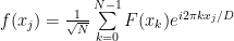
where D is the size of the space (in general it would be the volume, but here think of the 1D case only) and 
Its inverse transform (this is the actual transform to the ‘frequency’ space, the above being actually the ‘inverse’ transform back to the real space) is:

You’ll see later how this is useful in the case of the current topic, but in general, a good suggestion would be to look into using this when you notice a periodicity in the problem. For example, you’ll find periodicity in a crystal, where you have a basis cell repeated in the lattice. With Fourier transform you can switch to the reciprocal lattice which will ease computations. Sometimes even with no periodicity you can benefit from the plane wave basis decomposition by using a cell big enough with periodic boundary conditions.
The exponentials in the series terms have some nice properties, you can figure that immediately by hitting it with a differentiation or integral. You can see that way how a differential equation can turn into simple algebra. I hope I’ll have much more to say about this in future posts. By the way, since this post also handles a 2D problem and in the future 3D problems will be approached, solving a multi-dimensional Fourier transform is easy once you have the 1D transform. It’s easy to figure out that all you have to do is to do is to repeat the Fourier transform repeatedly for each dimension, the order has no importance. FFTW already has 2D and 3D transforms implemented, but for example for this project all I would have to do is to Fourier transform each row of the raw matrix then each column after that (or first the columns, then the rows), if only the 1D Fourier transform would be available.
Before finishing this, I want to mention that it’s not the first time you could see the expansion in a functions basis, it was already used in the Hartree-Fock project, but there a local basis was used, having our basis composed from Gaussians. Since the orbitals used were not orthogonal, the program had to deal with the overlap matrix and the generalized Eigen-value problem. Since plane waves are orthogonal, the overlap matrix is diagonal, so in an analogous problem one gets rid of the overlap matrix and deals only with the regular Eigen-value problem. More, the matrix elements there were quite hard to calculate. For the plane wave basis, one could find out that not only the matrix elements are easy to calculate but also operators that appear in the equation will be diagonal. This will ease up computations a lot, but there will be more about the details in future posts.
Nuclear Magnetic Resonance
Nuclear magnetic resonance is used for the magnetic resonance imaging so I thought I should at least point to some links here, I won’t enter much into details.
As the naming implies, the nuclear magnetic moment is the main ingredient in the method. Some nuclei do have spin. More, because the particles that compose a nucleus have charge, besides having each a 1/2 spin, they have a magnetic moment, too. The ‘have charge’ is more subtle than the net charge, because the neutron has no net charge, but still having 1/2 spin, it has a magnetic moment. This is because the quarks inside do have charge, despite adding to a zero net charge. The hydrogen nucleus, being a single proton, has a 1/2 spin. The nuclei that have both even number of protons and even number of neutrons, have no spin so they are not interesting for the subject. The reason if that the opposite spin identical in any other way will pair up in the same energy level, ending up with a zero spin for the nucleus. A nucleus with an odd number of protons and an odd number of neutrons will have an integer spin while for even-odd or odd-even numbers of protons and neutrons, respectively, the spin will be fractional (as in 1/2, 3/2 or 5/2). Of course the nuclear spin is quantified, too. If there is no magnetic field, there will be 2S+1 degenerate states, but if a magnetic field is added, the degeneracy is lifted.
If the magnetic field is on the z-axis direction, the energy difference between levels will be:

where g is the g-factor and 

Obviously, the atoms are not typically at zero temperature, so only some nuclei will be in the lower energy state, for the two levels of a 1/2 spin:

The magnetization is proportional with 


Imaging
I’ll try to describe a relatively simple method of having 2D (3D is also possible) magnetic resonance imaging. In practice there could be more complex, but you can find out more about that from the links.
Above I described how by applying a longitudinal homogeneous magnetic field, one could afterwards apply a transverse pulse that would turn into an absorption and later into emission in a very narrow frequency range corresponding to the resonant frequency. The emission intensity is determined by the nuclei concentration, but how do we find out the specific places where the signal originated?
You can select a particular plane by applying along the homogeneous magnetic field a longitudinal magnetic field gradient. This way a frequency value (a narrow range, actually) will correspond to a particular plane in the sample. If you apply the traversal 90 degrees pulse while having the gradient active, you’ll have only nuclei from the selected plane excited and precessing with the Larmor frequency. By the way, the pulse is specially crafted to have a narrow rectangular shape in frequency domain, so only a thin slice through the sample is excited.
After you apply the 90 degrees pulse, the longitudinal gradient is removed. If only this would be done, the evolution of nuclei from the slice would be with a precession with the same Larmor frequency. But if a transverse gradient is applied, the precession frequency will depend on the local magnetic field. After the gradient is eliminated, they will again precess with the common Larmor frequency, but they will have different phases, depending on the position along the transverse gradient. This results in a phase encoding. Measuring the phase will tell you where along the direction of the transverse gradient the signal originated. There is a problem, though, one needs two coordinates to locate a point in a plane! To solve this, another transverse gradient – in a direction perpendicular on the phase encoding one – is applied while measuring the signal. This results in a frequency encoding, since different positions along the second transverse direction correspond to different Larmor frequencies.
I will refer you to the image on top of this post, more specifically, the left image with the raw data. Imagine xOy coordinate axis with the (0, 0) point in the center of the image. The Ox axis corresponds to frequency encoding direction and the Oy one to the phase encoding. The frequency encoding is easier to understand, so I’ll explain first the data along the Ox axis (with y=0). In that case, there is no phase encoding gradient applied. Only the longitudinal plane selection gradient is applied along with the 90 degrees pulse to excite nuclei in the selected plane, then they are left to decay in a transversal frequency encoding gradient. While they are decaying the emitted signal is recorded. What you see on the Ox axis is the signal recorded, Ox is the time axis. Obviously the signal originates from points with different Larmor frequency, being the sum of all such signals. To separate out the frequencies and in consequence to obtain the position along the frequency encoding gradient, one has to do a Fourier transform. This separation still results in having a signal originating from all over the line perpendicular on the frequency encoding gradient direction, that is, a sum of all signals from the points along that line. To separate out the points one needs the phase encoding.
Phase encoding is a bit harder to grasp, so I will refer you to this page11. You don’t simply measure an absolute phase. What one can do is to measure relative phases. Typically one uses a reference signal to compare it with the measured signal. Forget about the fact that the signal is a sum of different frequencies, this is solved anyway by Fourier transforming the raw signal matrix rows, imagine you have a reference signal of a certain frequency and you have your measured signal of the same frequency but with a different phase. To keep things simple, imagine they have the same amplitude (if not, you can adjust one of them to have the same amplitude as the other). Using the reference signal you can find out the phase difference. The problem in the NMRI case is that you don’t have a reference signal but you have many signals (of the same frequency, after you separated out frequencies with the horizontal Fourier transform) with different phases, added up. You cannot extract the phase using a single such signal. The solution is to apply a different phase encoding gradient several times and record the signal as for the case with no phase encoding gradient. The difference can be either in the strength of the gradient, or you can apply the same gradient but for a longer and longer period of time. For the later case what you have on the vertical axis is the duration of the phase encoding gradient. For the negative Oy half-plane the phase encoding gradient is simply reversed.
So, after you used the Fourier transform on each line, you have the frequencies separated (which in turn separates out the distances in the Ox direction), but you still have a sum of different phases for the signal. To separate out the individual phases, one simply has to do the same Fourier transform in the phase encoding direction, by this also obtaining the distance along the gradient for phase encoding.
Conclusion
The goal of this post was to introduce the Fourier Transform and hint about some of its usages. I’ll refer to it in some other posts, where I won’t insist on Fourier transforms, I’ll consider that part as known. I’ll reuse the classes presented here is some other projects, perhaps improved, hopefully the changes won’t need any more explanations.
- FFTW The Fast Fourier Transform library. ↩
- Eigen The matrix library. ↩
- NMRI project on GitHub. ↩ ↩
- Fourier Transforms Lectures The playlist. ↩ ↩
- The Basics of MRI by Joseph P. Hornak. ↩ ↩ ↩
- The Basics of NMR by Joseph P. Hornak. ↩ ↩ ↩
- GPU Gems 2 CD Source tree with the data file. ↩
- GPU Gems 2 content ↩
- Chapter 48. Medical Image Reconstruction with the FFT from GPU Gems 2. ↩
- FFTW dlls Windows dlls download links and instructions. ↩
- What is phase encoding? Page about phase encoding on the MRI questions site. ↩
