Metropolis for 2D Ising and spin block renormalization

Introduction

After quite a bit of time, here is the C++ program I promised. I’ve made a youtube video just to present it, for more meaningful results it must run with way more sweeps than in the video:

It turned out that the program I used for making the video had some troubles with the frame rate and changes between frames and it couldn’t keep up so I had to cut out an interesting part, the evolution close to the critical temperature. Anyway, you can get the program yourself and run it, from here: Project on GitHub¹.

Theory

For theory I’ll send you again to the free computational physics book² I found on the net and also to a link into a CompPhysics GitHub repository, containing some lectures³ of Morten Hjorth-Jensen. Do browse the repository, you might find some interesting things there.

I already covered a bit of theory in Monte Carlo methods and The Ising Model posts so I won’t repeat it here. The implementation of the Metropolis Monte Carlo is very similar with the one from the previous post, just that now it’s in C++ instead of JavaScript and now there is an optimization by using pre-calculated values for the exponentials instead of calculating them each time. There is also some more in there, accumulating Energy and Magnetization to be able to calculate statistics. Here is the code for a Monte Carlo sweep, for comparison:

void SpinMatrix::MonteCarloSweep()
{
    unsigned int size = m_rows * m_cols;

    std::uniform_int_distribution<unsigned int> rndRow{ 0, m_rows - 1 };
    std::uniform_int_distribution<unsigned int> rndCol{ 0, m_cols - 1 };

    std::uniform_real_distribution<double> dbl_dist{ 0 , 1 };

    for (unsigned int pos = 0; pos < size; ++pos)
    {
        unsigned int row = rndRow(rndEngine);
        unsigned int col = rndCol(rndEngine);

        double energyDif = EnergyDifForFlip(row, col);
        if (energyDif < 0)
        {
            // accept it
            // flip the spin
            m_spins[m_cols*row + col] *= -1;
            Energy += energyDif;
            Magnetization += 2 * GetSpin(row, col);
        }
        else
        {
            //double val = ExpMinusBetaE(energyDif);
            double val = expMap[(unsigned int)energyDif];

            if (dbl_dist(rndEngine) < val)
            {
                // accept it
                // flip the spin
                m_spins[m_cols*row + col] *= -1;
                Energy += energyDif;
                Magnetization += 2 * GetSpin(row, col);
            }
            // else reject it, which means do nothing
        }
    }
}

void SpinMatrix::MonteCarloSweep()

{

unsigned int size = m_rows * m_cols;

std::uniform_int_distribution<unsigned int> rndRow{ 0, m_rows - 1 };

std::uniform_int_distribution<unsigned int> rndCol{ 0, m_cols - 1 };

std::uniform_real_distribution<double> dbl_dist{ 0 , 1 };

for (unsigned int pos = 0; pos < size; ++pos)

{

unsigned int row = rndRow(rndEngine);

unsigned int col = rndCol(rndEngine);

double energyDif = EnergyDifForFlip(row, col);

if (energyDif < 0)

{

// accept it

// flip the spin

m_spins[m_cols*row + col] *= -1;

Energy += energyDif;

Magnetization += 2 * GetSpin(row, col);

}

else

{

//double val = ExpMinusBetaE(energyDif);

double val = expMap[(unsigned int)energyDif];

if (dbl_dist(rndEngine) < val)

{

// accept it

// flip the spin

m_spins[m_cols*row + col] *= -1;

Energy += energyDif;

Magnetization += 2 * GetSpin(row, col);

}

// else reject it, which means do nothing

}

Obtaining information

As you can see in the code above, energy and magnetization are needed. There are two options: either calculate energy and magnetization when needed by summing up for all spins, or calculate it only once and then only modify the values each spin flip. If you want to use for statistics the state obtained after each sweep, the second method is better because not all spins are flipped during a sweep, some flips are rejected by the algorithm, so the computational cost is lower when using the latter method.

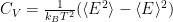
Getting the average energy and magnetization is straightforward, to get the specific heat and susceptibility a little bit more work is needed. For the specific heat:

$C_V = \frac{\partial \langle E\rangle}{\partial T}$

The average energy is given by:

$\langle E\rangle=\frac{1}{Z}\sum\limits_i E_i e^{-\beta E_i}$

Z is the partition function and plays an important role in statistical physics:

$Z=\sum\limits_i e^{-\beta E_i}$

Substituting in the formula for the specific heat and calculating derivatives one gets, after some calculations which I’m too lazy to type:

$C_V = \frac{1}{k_B T^2} (\langle E^2\rangle - \langle E\rangle^2)$

It works in a similar manner for every pair of conjugate variables, in this case for susceptibility one gets:

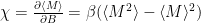
$\chi = \frac{\partial \langle M\rangle}{\partial B} = \beta (\langle M^2\rangle - \langle M\rangle^2)$

By the way, in the code the Boltzmann constant is set to 1, the same goes for J. The reason why J appears explicitly in the code is to allow for further change of the code, to try out anti-ferromagnetic interaction, too.

Here is the code that gets the specific heat into the chart, the one for the magnetic susceptibility is quite similar:

void CIsingMonteCarloDoc::SetupSpecificHeatChartData()
{
    std::vector<std::pair<double, double>> data;
    data.reserve(statsList.size());

    for (auto &&stat : statsList)
    {
        double val = abs(stat.AvgE2 - stat.AvgE * stat.AvgE) / (stat.Temperature * stat.Temperature * opt.latticeSize * opt.latticeSize);
        data.push_back(std::make_pair(stat.Temperature, val));
    }

    m_specificHeatChart.clear();
    m_specificHeatChart.AddDataSet(&data, (float)opt.chartLineThickness, opt.specificHeatColor);
}

void CIsingMonteCarloDoc::SetupSpecificHeatChartData()

{

std::vector<std::pair<double, double>> data;

data.reserve(statsList.size());

for (auto &&stat : statsList)

{

double val = abs(stat.AvgE2 - stat.AvgE * stat.AvgE) / (stat.Temperature * stat.Temperature * opt.latticeSize * opt.latticeSize);

data.push_back(std::make_pair(stat.Temperature, val));

}

m_specificHeatChart.clear();

m_specificHeatChart.AddDataSet(&data, (float)opt.chartLineThickness, opt.specificHeatColor);

}

Spin block renormalization

For some info on the spin block renormalization I simply refer you to Real Space Renormalization Group Techniques and Applications by Javier Rodriguez-Laguna⁴.

I just want to mention here some details about the implementation: although I could implement a majority rule for 3×3 spin blocks, I chose to use 2×2 for visualization reasons. This way there is an ambiguity, because some blocks might have no magnetization. In such a case it is customary to use a random value, I chose to use decimation instead by just picking the upper left corner value to decide. For the decimation alternative, I used the same upper-left value, sometimes the deciding spin is picked at random. The code can be easily changed to use any variant, feel free to experiment.

Since the spin block renormalization group originated with the work of Leo Kadanoff, which sadly passed away last year, I’ll point to a recorded statistical mechanics lecture presented by Kadanoff at Perimeter institute⁵.

To get some interesting results for the renormalization, one should make calculations for quite a big spin matrix size and also have one of the temperatures at the critical temperature (which is a little bit higher than the theoretical one for an infinite size system). A state under the critical temperature will evolve during renormalization transform towards the T=0 fixed point, while one above the critical temperature will evolve towards the infinite temperature fixed point. Those are relatively easy to obtain. A state that’s at the critical temperature will exhibit a scale invariance, that is, it will look more or less similar no matter how much the system is ‘zoomed out’ (not exactly true for the finite system, whence the need of using a big matrix for visualization).

I’ll try to record a video later with a big matrix size as an example and post it here.

Possible improvements

I had to stop without complicating the program too much, or else it could take a long time to have a program for the blog post. In the links I provided there is information about error estimation and improvement in statistics calculation.
A simple improvement to avoid autocorrelation would divide the results into blocks, average them for each block and use the averages for calculations (this is also called the binning method). The Computational Physics book² treats it along with the jackknife and bootstrap methods.
To avoid the critical slowdown close to the critical temperature, the heat bath method or a clustering algorithm like Wolff algorithm could be used, too.
Parallelization can be also improved, I chose the easiest way to parallelize it: just run independent threads and gather statistics from all of them. One can divide the spin matrix into stripes or even blocks and run the algorithm in parallel on the same spin matrix (not with different spin matrices as this project). The algorithm can be implemented with OpenCL or CUDA to run on the video card, for example.

Results

Here are some charts I got by running with seven threads and with many sweeps (thousands) for equilibration and over 10000 for statistics, for a 128×128 spin matrix. The temperature step was 0.05.

The Code

Before presenting the classes, a little bit of a rant. I displayed the spins first with GDI+ calls – FillRectangle. I have a pretty decent monitor so it’s quite a bit of resolution. With the application maximized, the frame rate achievable was very low. One would expect more from a dual Xeon workstation and a pretty decent video card (although with passive cooling). I ‘downgraded’ to simple GDI to learn that there is no much of a difference, which I expected, but I had to try… then I switched to Direct2D, although I hate using it with mfc because print preview does not work with it (I did use it in the electric field lines project, though, just for fun). It appeared to be faster, but not much faster. I did not time it until that point, so I cannot say what was the difference, but it was pretty small. I turned back at the plain old GDI and used a bitmap instead. More precisely, a memory device independent bitmap (DIB). You can get more speed by using a device dependent one (I did even that in the past) but it’s not worth it. The big speed jump (as in from 2 frames/second to 50 frames/second or more) was due of avoiding calls into the slow library and implementing the equivalent call into my own class. Probably using device dependent bitmaps would make it a little bit faster and using Direct2D even faster, but just a little bit. Not worth it.

So, here are the classes in the order of importance (sort of):

SpinMatrix – More or less similar with what I presented in the previous post, but with the addition of pre-calculating the exponential values and with renormalization code added. It can be initialized at ‘zero’ temperature or infinite temperature. It’s just the spin matrix with periodic boundary conditions, containing the implementation of a Metropolis Monte Carlo sweep on the spins.

MonteCarloThread – Has a SpinMatrix member called spins. In Calculate it runs a TemperatureStep for each temperature in the interval, starting with the lower one. Before this loop it runs a ‘warmup’ loop. The TemperatureStep just runs several sweeps for equilibration then several others for gathering statistics. The numbers are configurable, of course. One thread will pass the spin matrix to the main thread for displaying – in PassData, all threads will gather statistics in PassStats.

Statistics – Contains the accumulated statistics and has some operators overloaded and a CollectStats method. The usage is pretty straightforward.

CIsingMonteCarloDoc – The document class. Manages the threads, the data gathering and the spin matrices for display – both the ones that are displayed during threads running and when displaying the spin block renormalization. It also handles the charts and chart data. It has a copy of Options because the options that are stored in the application object can change during threads running.

MemoryBitmap – The class that helps with displaying the spin matrix. Plain old GDI for drawing, nothing fancy.

CIsingMonteCarloView – the view. Has a timer, deals with displaying and printing. Also holds some MemoryBitmap members for displaying.

Chart – The charting class. I just copied it from the nrg project. It uses GDI+ for drawing.

Options – The options class, it has methods to save them into registry and load them from registry.

COptionsPropertySheet, CIsingModelPropertyPage, CSimulationPropertyPage, CRenormalizationPropertyPage, CDisplayPropertyPage, CChartsPropertyPage, the property sheet class and the property pages classes, respectively. Quite standard mfc implementations, nothing hard to understand.

CNumberEdit – the edit control for double/float values. I just copied it from the nrg project.

ComputationThread – the base class for MonteCarloThread.

CMainFrame – the main frame. Deals with menu commands.

CIsingMonteCarloApp – the application class. Has an Option member, loads the options at startup and also deals with GDI+ initialization.

CAboutDlg – what the name says.

Conclusion

This concludes for now the posts about the Monte Carlo methods, hopefully I’ll have more posts about them in the future, but I’ll probably switch to something else next post.

If you notice and issues, bugs, mistakes and so on, please let me know. As a warning, I did not test the magnetic field at all so the code might be buggy with a non-zero magnetic field.
CodeProject

IsingMonteCarlo Project on GitHub. ↩
Computational Physics A book by Konstantinos Anagnostopoulos. ↩ ↩
2015 lectures by Morten Hjorth-Jensen. ↩
Real Space Renormalization Group Techniques and Applications by Javier Rodriguez-Laguna. ↩
Statistical Mechanics lecture by Leo Kadanoff. ↩

Metropolis for 2D Ising and spin block renormalization

Introduction

Theory

Obtaining information

Spin block renormalization

Possible improvements

Results

The Code

Conclusion

Like this:

Related

Leave a Reply (for privacy concerns, please read the Privacy Policy Page accessible from the top menu)Cancel reply

Introduction

Theory

Obtaining information

Spin block renormalization

Possible improvements

Results

The Code

Conclusion

Share this:

Like this:

Related

Leave a Reply (for privacy concerns, please read the Privacy Policy Page accessible from the top menu)Cancel reply