
Introduction
Quite a bit of time passed since my last post on this blog. I had a visit to the sunny Spain, I switched to a double-surface hang glider and I had to take a little care of my firm. Despite those things, I did a little bit of work for the blog, but it took me a little longer than I anticipated. This is a first post of ‘theory’ before presenting the code I implemented. If you want to take a look before having the description available, here it is: a Hartree-Fock program1. I posted the project on GitHub a couple of weeks ago, but I just didn’t have the patience to start writing about it.
This post will be more general, not addressing the project much, but I hope I’ll refer it in more than one post, so here it is. It’s just an opportunity to collect together some links for those that need more info than the one that will be exposed in the next post, than a detailed description.
The Problem
The problem appears to be simple, you have a bunch of particles, you want to see what happens to them. They might be some protons and neutrons in a nucleus, or a nucleus and the electrons in an atom, or more than one nucleus and more electrons forming a molecule. Or even larger systems, forming nanostructures or even crystals. The problem turns out to be very complex because they are interacting. A problem with more than two particles interacting – even with relativity dropped – cannot be solved exactly, you’ll have to resort to simplifications in order to obtain approximate solutions. The first simplification is to drop out relativity. With the Schrödinger equation, one can take relativity into account, but I’ll simply ignore it for now. The Hamiltonian for such a system is:

where K is the kinetic energy term and V is the potential energy term. The potential energy can be a sum of internal potential energy and external potential energy, because of an external field. The external field might be time dependent, which would complicate things a bit. From now on, unless explicitly stated, I’ll consider the external potential to be zero. This is the second simplification. Now, let’s switch to the equation that deals with such a system.
Schrödinger equation
With no more words, here it is:

where:

I deliberately did not detail yet the dependency of 
Don’t forget about the simplifications we use, if you want to consider an external magnetic field, too, for example, check out the Schrödinger–Pauli equation.
You may ‘justify’ the equation by taking a plane wave and hit it with time and position partial derivatives, trying to form the operators and arrange them in such a way to get the wave equation. You’ll also need to consider the de Broglie hypothesis, 

The equation is a linear equation. This means that if you have two solutions for the equation, any linear combination of them is also a solution. So it’s not only a plane wave that is a solution for the equation, but you may also compose wave packets out of them that are also solutions.
If the Hamiltonian does not depend explicitly on time, one can use separation of variables to find stationary solutions of the equation. One obtains the time independent Schrödinger equation:

Don’t forget that the wave function still evolves in time, the time evolution operator being 

Since we got rid of external potentials (and that includes those that vary in time) wanting to simplify the problem as much as possible, we’re from now on considering the time independent equation, the time dependency being trivial. We’re going to use another simplification, to get rid of all sorts of constants that complicate the formulae, that is, we’re using the atomic units.
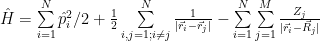
The Hamiltonian for our bunch of particles being nuclei and electrons in a molecule is:

N is the number of electrons, M the number of nuclei, Z is the atomic number. The first two terms are the kinetic energy terms for electrons and nuclei, respectively, the next ones being in order: the electron-electron repulsion potential energy, the electron-nucleus attraction energy term and the nucleus-nucleus repulsion energy term. The interaction is nothing more than the plain old Coulomb interaction.
It looks complicated and it’s even way more difficult to solve than the looks might suggest. For a single nucleus and one electron only it can be solved analytically but even that is not exactly easy. Having a bunch of electrons and nuclei creates a problem that is analytically intractable. Even if you try to solve it as it is using some naive numerical approach, it’s not easy solvable even for four particles. Can we simplify it even more?
Born–Oppenheimer approximation
Yes we can, but this will only approximate the solution to the complete equation. The approximation turns out to be very good in many cases, so here it is. It is based on the observation that the electrons are very light compared with nuclei. Even compared with a single proton, the electron is more than 1800 times lighter. As a consequence, the nuclei ‘move’ much slower than the electrons, the electronic cloud adjusting to the nuclei configuration almost instantly. This allows separation of the motion of nuclei from the Schrödinger equation, you may treat them separately even using a classical approach. With the Born–Oppenheimer approximation the Hamiltonian we’ll have to solve first becomes:
that is, we eliminated the nuclei kinetic energy term and the nucleus-nucleus repulsion energy term, which remain to be handled separately. We have now only the electrons kinetic energy term, the electron-electron interaction term and the electron-nucleus interaction term.
Representations, notations, formalism and so on…
Obviously I cannot enter into details here, I cannot write an entire quantum physics book in a blog post. There are plenty of books, there are plenty of resources on internet, too. I already pointed the Feynman lectures vol III2, I will point out another resource, chosen arbitrarily: Quantum Mechanics, by Richard Fitzpatrick3.
There are (or will be, hopefully) posts on this blog that might require you to be familiar with the Dirac notation, with various representations, the different ‘pictures’ (Schrödinger picture, Heisenberg picture, interaction picture), second quantization, Hilbert space, Fock space and so on… Unfortunately you’ll either have to be familiar with those – in which case there is a low probability that you need to read this post 🙂 – or be willing to look yourself into them, I cannot explain them all here. I’m trying to keep things simple and give links to more details but this is not always possible.
When I started writing this post I wanted to give some details in this paragraph about the relationship between matrix mechanics and the wave formulation and also about some things linked above and maybe more, but I realized that it would be way too much to write than I’m willing and have patience to do, so I’ll let it as it is. Maybe some other time… but I must warn you that you’ll see a lot of matrices in the quantum mechanics related programs (and not only there, the matrix representation is very useful).
Exact diagonalization
This is another way one could try to attack the problem. Unfortunately it’s not very useful for complex systems, because of the exponential increase of the vector space. That does not mean it’s not useful, a quick google search might reveal a lot of hits. This is just the first hit I got: Exact Diagonalization, being a part of a Quantum Simulation course4. I thought that at least the method should be mentioned here.
Variational principle
Ok, so we reached the important part, the variational principle. It’s used not only in the Hartree-Fock method about which I already have the program on GitHub1, but in many other cases, for example in Variational Quantum Monte Carlo or Density Functional Theory. I intend to make some programs that use the two mentioned methods for this blog, by the way.
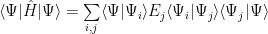
This principle is so important for this post that the image on top contains an important formula. It’s the energy functional, with the wave vector assumed normalized. I think that the Wikipedia page is quite a good start, but anyway, I’ll detail a part here, too. Let’s start with the right hand side of the energy functional:

There is nothing fancy going on, just the unit operator being inserted twice. It’s the superposition principle in action, if you have a particular basis for your vector space, you may decompose/write your vector using its projections on the vectors that form the basis:

with the component along a particular basis vector being not surprisingly, the projection onto that vector (that is, the scalar product between them):

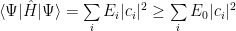
So, the Hamiltonian acting on an eigenvector gives the eigenvalue (by the way, we use the energy eigenvectors as basis):
But the eigenvectors are orthogonal, so:

Obviously, using the smallest energy from the spectrum, that is, the ground state energy, we find:
The ground state energy is just a constant, it can be taken out of the sum and using the fact that the wave vector is normalized, one gets:
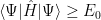
Ok, but what does it mean? It means that no matter what wave function we try, we’ll get an energy that is bigger than the ground state energy (or equal, if we manage to pick up the ground state – or a ground state, if there are more of them).
If we try one at random, we get one expectation value. By some method we pick another wave function and calculate the expectation value for it. If it’s smaller, we drop the first guess and keep the new one. We can repeat the trials until hopefully we are close enough to the ground state. How we pick the state and how we modify it depends on the particular method and I’ll detail it for the specific program.
If you want to find more about this, here is a link: Introduction to Electronic Structure Calculations: The variational principle5.
I should also mention here that you could derive the time independent Schrödinger equation by using variational calculus and imposing that a stationary state has the energy variation vanishing in the first order if the wave vector suffers a small variation 
Perturbation theory
I want to mention perturbation theory here, because I might use it in a future project for this blog. Not only that, but related with the following subject, Hartree-Fock, it can be used for a Post Hartree-Fock improvement, see Møller–Plesset perturbation theory.
Since we assumed that the Hamiltonian we have to deal with is not explicitly time dependent, I’ll let aside for now the time-dependent perturbation theory. If ever needed for this blog, I’ll detail it there.
The time independent perturbation theory is detailed well on the linked Wikipedia page, I want to emphasis here just the main ideas. In the case you have a Hamiltonian that you cannot solve, but you can write it as a sum of a Hamiltonian that can be solved (either exactly or by some approximation method) and a small term, then you can use the perturbation theory to get an approximate solution for the whole Hamiltonian. You need to expand both the eigenstates and eigenvalues of the full Hamiltonian in Taylor series at the unperturbed eigenstate/eigenvalue and substitute them into the time independent Schrödinger equation. Expanding and identifying the terms that have the same power allows you to get the correction terms. Obviously one has to stop at a certain order, when the approximate solution is close enough to the real one.
Conclusion
We ended up with a Hamiltonian which is still quite complex and very hard to solve even for simple systems. If we could simplify somehow the interaction terms we could try to solve it, but as it is it’s still very difficult. There are various ways of doing that, but that’s a subject for other posts.
So that’s it for now. The next post will be about Hartree-Fock theory. Then another one will follow that will present the program1
- A Hartree-Fock program The project on GitHub. ↩ ↩ ↩
- Feynman lectures Vol III, Chapter 16, The Dependence of Amplitudes on Position. ↩ ↩
- Quantum Mechanics by Richard Fitzpatrick. ↩
- Quantum Simulation course at Institute for Theoretical Physics – Weimer Group, Lecturer: Dr. Hendrik Weimer. ↩
- Introduction to Electronic Structure Calculations: The variational principle by Ivo Filot. ↩
