Empirical Pseudopotential

Introduction

I did not write anything on the blog for a long time. I was very busy, I had less time for it. Nevertheless, I did some work on some projects related with it. One of them, a DFT program that calculates a molecule with the supercell method, was supposed to be the theme for a blog entry. I implemented it, it works (sort of) but it needs some checks and cleanup. I implemented it with local pseudopotentials, specified in real space, one which I generated from the Ge one given in the references I mentioned in the last posts and some more which I found on the internet. Unfortunately it doesn’t give results as good as I expected. I might want to change it to use nonlocal pseudopotentials.

I also modified the Hartree-Fock project to be able to calculate and display the dissociation energy and the ionization energy, using Koopmans’ theorem, so in fact it’s the last energy level. I did this mainly because I wanted to compare some results with the DFT molecule program, the dissociation energy computed with Hartree-Fock cannot be very good. Another project I modified a little was the Lattice Boltzmann one, I tried to improve its speed a little.

What I wanted to have in the end with all those DFT projects is to use it in computations for crystals. So, since I postponed that project indefinitely, I thought I should at least have another project with pseudopotentials. Something much simpler than DFT. But before going to discuss that project, here is a result that is also presented in the lectures I pointed out in the last blog entries:

110 section through Ge crystal, computed with DFT with pseudopotentials

This is obtained with the Octave code, although I can reproduce the results with the C++ code from the molecule computation project.

Now, back to the subject of this blog post: a project that computes the band structure of a crystal having the diamond/zincblende structure, for various elements. The project is already on GitHub: Empirical Pseudopotential¹, it was there for a while before writing this. Actually, there is already another project on GitHub which also misses description here, but about that one, later.

As usual, here is the program in action, in a YouTube video:

Some theory

Since this is such an easy subject I will resume to providing some Wikipedia links for visitors that are not familiar with the concepts and then some links to some pdfs dealing with the subject, then I will only very briefly write some words about the theory.

Wikipedia links

You should be familiar with the Bravais lattice. The fact that we’re dealing with a periodic infinite structure allows us to study it by applying Fourier theory, so you should also understand how the Reciprocal lattice is used. It’s not merely a mathematical trick, the reciprocal vectors have a direct correspondence with scattering vectors from diffraction on a crystal lattice. Bloch waves play a very important role in studying crystals, so you should be familiar with those, too. Once you understand how a particular Bloch wave can have different decompositions, you should understand why we can restrict to studying only the first Brillouin zone.

Some papers

The program is based on parameters given in Band Structures and Pseudopotential Form Factors for Fourteen Semiconductors of the Diamond and Zinc-blende Structures by Marvin L. Cohen and T. K. Bergstresser² so I thought I should reference it first. One pdf that describes the theory very nicely is on nanohub: Empirical Pseudopotential Method by Dragica Vasileska³. A master thesis containing both theory and C code is: Empirical pseudopotential method for modern electron simulation by Adam Lee Strickland⁴. If you grasp the theory you may want to apply the method on some other materials, with some other structure, like graphene. For such a case, here is a master thesis dealing with it: Band Structure of Graphene Using Empirical Pseudopotentials by Srinivasa Varadan Ramanujam⁵. Those links should be enough, if not, google should be able to reveal more related with the subject.

Very brief theory

We’ll start with the uni-electron Schrödinger equation:

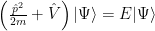
$\left(\frac{\hat{p}^2}{2m} + \hat{V}\right)|\Psi\rangle = E |\Psi\rangle$

With it, we are describing non-interacting electrons moving into the potential of the atomic nuclei in the crystal. Of course, the problem is a many-body problem and often you cannot get away with such simplification, but sometimes even the free electron model can be good enough, or at least the nearly free electron model, so it’s worth a try.

We can benefit from having a periodic arrangement of atoms. Because the Hamiltonian commutes with all discrete translation operators, we can pick common eigenvectors to describe the solutions, namely Bloch vectors. A Bloch function has the form:

$\Psi_{n,\vec{k}}\left(\vec{r}\right) = u_n(\vec{k}) e^{i \vec{k}\vec{r}}$

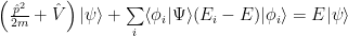
We can avoid the ambiguity of decomposing in the plane wave and the periodic function u by limiting to the first Brillouin zone. Since electrons close to nuclei are deep in the potential well of the nucleus, they are perturbed very little by the potentials of the other nuclei and they cannot easily tunnel out (that is, they are not so ‘free’ as the electrons we are trying to describe), so we can describe them using linear combination of atomic orbitals. A problem is that the Bloch functions are not orthogonal on the atomic orbitals. That would force us to use the overlap matrix and have to deal with the generalized eigenvalue problem. Alternatively, we can orthogonalize the ‘plane waves’ by the usual procedure: extract from vectors the projections of the vector along all the others:

$|\psi\rangle = |\Psi\rangle - \sum\limits_{i} \langle \phi_i | \Psi \rangle | \phi_i \rangle$

where $| \phi_i \rangle$ are the atomic orbitals. It’s easy to get from this the original wavevector and substitute it into the Schrödinger equation:

$\left(\frac{\hat{p}^2}{2m} + \hat{V}\right)\left( |\psi\rangle + \sum\limits_{i} \langle \phi_i | \Psi \rangle | \phi_i \rangle \right) = E \left( |\psi\rangle + \sum\limits_{j} \langle \phi_j | \Psi \rangle | \phi_j \rangle \right)$

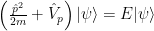
Applying the Hamiltonian operator on each term and moving the second right term to the left we get:

$\left(\frac{\hat{p}^2}{2m} + \hat{V}\right) |\psi\rangle + \sum\limits_{i} \langle \phi_i | \Psi \rangle (E_i - E) | \phi_i \rangle = E |\psi\rangle$

We can force it back to Schrödinger equation:

$\left(\frac{\hat{p}^2}{2m} + \hat{V} + \sum\limits_{i} \langle \phi_i | \Psi \rangle (E_i - E) \frac{| \phi_i \rangle}{|\psi\rangle} \right)|\psi\rangle = E |\psi\rangle$

Call the repulsive term $\sum\limits_{i} \langle \phi_i | \Psi \rangle (E_i - E) \frac{| \phi_i \rangle}{|\psi\rangle} = \hat{V}_R$ and notice that we still have a Schrödinger equation with the same eigenvalues but different eigenvectors, having not only the attractive potential given by the nucleus, but also a repulsive potential given by the core electrons. Call $\hat{V}_p = \hat{V} + \hat{V}_R$ the pseudopotential and we have to solve:

$\left(\frac{\hat{p}^2}{2m} + \hat{V}_p\right)|\psi\rangle = E |\psi\rangle$

The only problem that remains apart from solving it is to determine the pseudopotential. You have various means for that, from computing it to determining it from experimental results. I’ll let you find the details from the given links…

The code

If you are interested only in the computations, all the relevant classes – except Vector3D which was already used in many projects for this blog – are in the EmpiricalPseudopotential namespace. SymmetryPoint is a class for a very simple object: it has only a ‘name’ and a position in the reciprocal space. SymmetryPoints contains a map of such objects. Its constructor just initializes it with the critical points of the face-centered cubic lattice. SymmetryPoints::GeneratePoints generates the points that are charted. You pass it a ‘path’ formed by symmetry points and the number of desired points to have in the chart and it computes the k-points coordinates. It also returns the indices of the symmetry points in symmetryPointsPositions. The Material class is also simple, it’s for objects that store a material name, a distance in Bohrs between the basis cell atoms and the pseudopotential. There is a Materials class that just holds a map of materials. The map is filled in the constructor, a configuration file would be probably a better alternative, but for the purpose of this project, it’s good enough. By the way, you’ll see some conversions going on there, it’s because the parameters were given in Angstroms and Rydbergs, but computations are done in Hartree atomic units.

The Pseudopotential just holds the parameters for a pseudopotential and has a single function:

std::complex<double> Pseudopotential::GetValue(const Vector3D<int>& G, const Vector3D<double>& tau) const
{
    const int G2 = G * G;
    const double Gtau = 2. * M_PI * tau * G;

    double VS = 0;
    double VA = 0;

    if (3 == G2)
    {
        VS = m_V3S;
        VA = m_V3A;
    }
    else if (4 == G2)
    {
        VA = m_V4A;
    }
    else if (8 == G2)
    {
        VS = m_V8S;
    }
    else if (11 == G2)
    {
        VS = m_V11S;
        VA = m_V11A;
    }

    return std::complex<double>(cos(Gtau) * VS, sin(Gtau) * VA);
}

std::complex<double> Pseudopotential::GetValue(const Vector3D<int>& G, const Vector3D<double>& tau) const

{

const int G2 = G * G;

const double Gtau = 2. * M_PI * tau * G;

double VS = 0;

double VA = 0;

if (3 == G2)

{

VS = m_V3S;

VA = m_V3A;

}

else if (4 == G2)

{

VA = m_V4A;

}

else if (8 == G2)

{

VS = m_V8S;

}

else if (11 == G2)

{

VS = m_V11S;

VA = m_V11A;

}

return std::complex<double>(cos(Gtau) * VS, sin(Gtau) * VA);

}

It’s quite simple because we need values only in some points, over 11 for $G^2$ the value can be very well approximated with 0 and for $G^2=0$ the value can be set to zero being only a shift in energy.

All the above mentioned classes should be very easy to understand. I have only two of them left to describe, both being important. First, one for the Hamiltonian:

class Hamiltonian
{
public:
    Hamiltonian(const Material& material, const std::vector<Vector3D<int>>& basisVectors);

    void SetMatrix(const Vector3D<double>& k);
    void Diagonalize();

    const Eigen::VectorXd& eigenvalues() const { return solver.eigenvalues(); }
protected:
    const Material& m_material;
    const std::vector<Vector3D<int>>& m_basisVectors;

    Eigen::MatrixXcd matrix;

    Eigen::SelfAdjointEigenSolver<Eigen::MatrixXcd> solver;
};

class Hamiltonian

{

public:

Hamiltonian(const Material& material, const std::vector<Vector3D<int>>& basisVectors);

void SetMatrix(const Vector3D<double>& k);

void Diagonalize();

const Eigen::VectorXd& eigenvalues() const { return solver.eigenvalues(); }

protected:

const Material& m_material;

const std::vector<Vector3D<int>>& m_basisVectors;

Eigen::MatrixXcd matrix;

Eigen::SelfAdjointEigenSolver<Eigen::MatrixXcd> solver;

};

You may recognize there the material for which the Hamiltonian is constructed, the basis vectors that are used for matrix representation of the Hamiltonian, the actual Hamiltonian matrix and the solver used to diagonalize it.
You may look in the project sources¹ for the full implementation, here is the one for `SetMatrix’:

void Hamiltonian::SetMatrix(const Vector3D<double>& k)
{
    const unsigned int basisSize = static_cast<unsigned int>(m_basisVectors.size());

    for (unsigned int i = 0; i < basisSize; ++i)
        for (unsigned int j = 0; j < i; ++j) // only the lower triangular of matrix is set because the diagonalization method only needs that
            // off diagonal elements
            matrix(i, j) = m_material.pseudopotential.GetValue(m_basisVectors[i] - m_basisVectors[j]);

    for (unsigned int i = 0; i < basisSize; ++i)
    {
        // diagonal elements
        // this is actually with 2 * M_PI, but I optimized it with the /2. from the kinetic energy term
        const Vector3D<double> KG = M_PI / m_material.m_a  * (k + m_basisVectors[i]);

        matrix(i, i) = std::complex<double>(2. * KG * KG); // 2* comes from the above optimization, instead of a /2
    }
}

void Hamiltonian::SetMatrix(const Vector3D<double>& k)

{

const unsigned int basisSize = static_cast<unsigned int>(m_basisVectors.size());

for (unsigned int i = 0; i < basisSize; ++i)

for (unsigned int j = 0; j < i; ++j) // only the lower triangular of matrix is set because the diagonalization method only needs that

// off diagonal elements

matrix(i, j) = m_material.pseudopotential.GetValue(m_basisVectors[i] - m_basisVectors[j]);

for (unsigned int i = 0; i < basisSize; ++i)

{

// diagonal elements

// this is actually with 2 * M_PI, but I optimized it with the /2. from the kinetic energy term

const Vector3D<double> KG = M_PI / m_material.m_a * (k + m_basisVectors[i]);

matrix(i, i) = std::complex<double>(2. * KG * KG); // 2* comes from the above optimization, instead of a /2

}

If you looked over the theory, you’ll recognize the formulae immediately.

The last one is BandStructure, a little more complex but not a big deal. AdjustValues just converts Hartees to eV and shifts the energy value to a zero which is found with FindBandgap. Initialize is straightforward, GenerateBasisVectors just fills basisVectors with vectors that have the proper length (that length squared is in G2).

Here is the Compute function:

std::vector<std::vector<double>> BandStructure::Compute(const Material& material, unsigned int startPoint, unsigned int endPoint, unsigned int nrLevels, std::atomic_bool& terminate)
{   
    std::vector<std::vector<double>> res;

    Hamiltonian hamiltonian(material, basisVectors);

    for (unsigned int i = startPoint; i < endPoint && !terminate; ++i)
    {
        hamiltonian.SetMatrix(kpoints[i]);
        hamiltonian.Diagonalize();

        const Eigen::VectorXd& eigenvals = hamiltonian.eigenvalues();

        res.emplace_back();
        res.back().reserve(nrLevels);

        for (unsigned int level = 0; level < nrLevels && level < eigenvals.rows(); ++level)
            res.back().push_back(eigenvals(level));
    }

    return std::move(res);
}

std::vector<std::vector<double>> BandStructure::Compute(const Material& material, unsigned int startPoint, unsigned int endPoint, unsigned int nrLevels, std::atomic_bool& terminate)

{

std::vector<std::vector<double>> res;

Hamiltonian hamiltonian(material, basisVectors);

for (unsigned int i = startPoint; i < endPoint && !terminate; ++i)

{

hamiltonian.SetMatrix(kpoints[i]);

hamiltonian.Diagonalize();

const Eigen::VectorXd& eigenvals = hamiltonian.eigenvalues();

res.emplace_back();

res.back().reserve(nrLevels);

for (unsigned int level = 0; level < nrLevels && level < eigenvals.rows(); ++level)

res.back().push_back(eigenvals(level));

}

return std::move(res);

}

kpoints is a vector of positions in the reciprocal space, previously generated in Initialize using SymmetryPoints::GeneratePoints. You can see above how the Hamiltonian class is used. The code just iterates between startPoint and endPoint, for each k-point the Hamiltonian matrix is set then it’s diagonalized, then the eigenvalues are retrieved and saved in results. startPoint and endPoint and terminate are used because the computation can be done with several threads.
For how that is done and how the data is put into a chart, you’ll have to look into the the project sources¹, mostly in the EPThread and EPseudopotentialFrame classes.

Options is for… options and OptionsFrame is the class that implements the options dialog box for editing them. EPseudopotentialApp is a very simple wxWidgets⁶ application class, wxVTKRenderWindowInteractor is a class that allows to easily use VTK⁷ from wxWidgets that I’ve got from here⁸ and modified it slightly to be able to compile with a more recent version of wxWidgets and that’s about it.

Libraries used

It should be obvious by now that I switched from mfc to wxWidgets⁶. I’ve got bored by mfc, although it’s easier to use with VisualStudio, but since they released a wxWidgets version that compiled with no issues on Windows, I decided to use it from now on with projects for this blog. The big benefit is that with minimal efforts the projects could be compiled to run not only on Windows, but on Linux or Mac as well. Since I switched to wxWidgets, to keep things portable I also had to avoid using my 2D charting class which I used in other projects. Instead of writing some new, portable code for a chart, I preferred to use VTK⁷ for the 2D chart.

As in many other projects, I also used Eigen⁹.

Conclusion

This concludes the presentation of the Empirical Pseudopotential project. If you find any issues, please let me know, either here or on GitHub.
Since I’m quite busy I might not post for a while here again, but there is already another project on GitHub, also for computing band structure, but using the tight binding method. The project is based on this project, I simply had to remove some code and change it into some places (obviously, for example the Hamiltonian had to be changed). The code is even simpler than the one of this project. In fact, it’s deceptively simple, the theory is not so simple if you go into the details.

CodeProject

Empirical Pseudopotential The project on GitHub ↩ ↩ ↩
Band Structures and Pseudopotential Form Factors for Fourteen Semiconductors of the Diamond and Zinc-blende Structures by Marvin L. Cohen and T. K. Bergstresser, Phys. Rev. 141, 789 – Published 14 January 1966 ↩
Empirical Pseudopotential Method by Dragica Vasileska ↩
Empirical pseudopotential method for modern electron simulation by Adam Lee Strickland ↩
Band Structure of Graphene Using Empirical Pseudopotentials by Srinivasa Varadan Ramanujam ↩
wxWidgets Cross-platform GUI library ↩ ↩
VTK, The Visualization Toolkit The scientific (and not only) visualization library ↩ ↩
wxVTK ↩
Eigen The matrix library. ↩

Introduction

Some theory

Wikipedia links

Some papers

Very brief theory

The code

Libraries used

Conclusion

Like this:

Related

Leave a Reply (for privacy concerns, please read the Privacy Policy Page accessible from the top menu)Cancel reply

Introduction

Some theory

Wikipedia links

Some papers

Very brief theory

The code

Libraries used

Conclusion

Share this:

Like this:

Related

Leave a Reply (for privacy concerns, please read the Privacy Policy Page accessible from the top menu)Cancel reply