Lattice Boltzmann

Introduction

It’s time for an easier topic than the last time. I noticed – but I also expected it – that I have more success with projects like the Solar System than with a project like the Numerical Renormalization Group. There are mainly two reasons for it: it looks more spectacular to see a 3D animation than a boring chart and the level required to understand it is lower. Those are some reasons why I’m going to have such easier and preferably nicely looking projects for this blog in the future, too. It also takes me much less time to implement such a project than a project as the Hartree-Fock one, for example.

So, the current topic is Lattice Boltzmann methods. The associated project is here¹. I already have it working for quite some time, but I had to implement the user interface, options and so on and I added some more boundary conditions for inlet and outlet, a little in a hurry and incomplete, but they should be enough to form an idea. In the meantime I took a short vacation and went to the annual Romanian hang gliding meeting, “Deltazaurii”, where I had a great time: part of a flight filmed from the crossbar.

The temptation to write a 3D one is big, what stopped me was first the 3D visualization which I don’t want to deal with currently and the amount of computation, which would require using the video card – with OpenCL or CUDA, but if I’ll decide to carry out something like this I would probably pick OpenCL. Even this project could use an OpenCL implementation, but the project would be a little harder to compile and also the code would be a bit less clear, so I gave up the idea.

It took very little time to have the algorithm working, just a bit more to have it multithreaded, most of the time was taken by refining displaying, adding the options, options property sheet and the additional boundary conditions for the inlet and outlet, where I became bored by the project so I rushed it out. One has to stop somewhere, or else developing a project on such a subject could take a lot of time. There are people that spent years developing projects related with subjects on this blog, obviously I cannot go into such depth if I want to have various topics on the blog and besides, such a project is very difficult to understand, which would be against the purpose of the blog.

Before entering into details, here is the program in action:

Links

This is a topic where I have no intention to present a lot of theory, so you might have to look into some other places for information on it. As usual, I’ll give some links here, but there is plenty more information to be found on the internet.
Here are a couple of papers I’ve looked into and I found to be enough to get the general idea: The Lattice Boltzmann Method for Fluid Dynamics: Theory and Applications², Implementation techniques for the lattice Boltzmann method³. I’ve heard good things about this one: The Lattice Boltzmann method with applications in acoustics⁴ although I very briefly looked over it. You should not stop there if you want more than this project covers, there is a lot to find out, there is a lot of work on thermal Lattice Boltzmann methods, a lot of work on boundary conditions, multi-phase flow and so on.

It’s not always advisable to write your own code – re-inventing the wheel – if you want to do some simulations, although my opinion is that for understanding the subject one should implement at least easy projects as this one before using some sophisticated library written by somebody else. If you want to use libraries, here are a couple of projects: OpenLB⁵, Palabos⁶. I’m sure you can find more…

The method

Very shortly, the idea for fluid dynamics simulation is to have some equations that model the fluid flow and solve them. They cannot be analytically solved except for very simple situations, so a numerical approach is used.
Those equations are obtained using some laws obeyed by the fluid, like conservation laws (mass conservation, momentum conservation, energy conservation). Historically, the fluid was considered a continuum medium and without more details, one had to solve Navier-Stokes equations, together with mass conservation, boundary conditions and perhaps energy conservation thrown in, perhaps with simplifying assumptions, like considering the fluid not compressible. One could attack the problem using at least the finite difference method but there are other methods that are used as finite element method, finite volume method and so on. I won’t detail much on this approach, I might decide to have something on this blog about either the finite element or finite volume method in the future, but not necessarily for fluid dynamics.

It should be obvious that the continuum hypothesis is actually false, we know that real fluids are composed of interacting particles (being atoms or molecules or more ‘exotic’ ones, like quark-gluon plasma). Of course it’s hopeless currently and for the foreseeable future to try to simulate such fluids ab initio for a typical fluid volume we need to simulate. We could observe that in some conditions some bigger particles (like sand) still behave like a fluid, so we could hope that even if making the particles big with some idealized interactions between them, we could get lucky and because of the universality we could get away and simulate the fluid flow using a much less number of particles than the fluid has. Historically, that was the method used, with Lattice Gas Automata. It had some issues so it was quickly replaced by the Lattice Boltzmann Methods.

The main idea is that instead of treating individual particles, a statistical physics approach is used. using distribution functions for particles. More specifically, it starts from Boltzmann equation which describes the behavior of the particles distribution at non equilibrium, involving collisions:

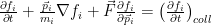
$\frac{\partial f_i}{\partial t} + \frac{\vec{p}_i}{m_i}\nabla f_i + \vec{F} \frac{\partial f_i}{\partial \vec{p}_i} = \left(\frac{\partial f_i}{\partial t}\right)_{coll}$

You can find the details about it either in the Wikipedia links or in the papers for which I provided the links already. The collision term can be quite complicated even with the “Stosszahlansatz”, making it a partial integro-differential equation quite hard to solve. The collision term is typically simplified further, using a relaxation time $\tau$ , the collision term becoming $\frac{f_{0i} - f_i}{\tau_i}$ . In general, if you have a mix of different fluid phases, different phases have different relaxation times.

You’ll find the mathematical details of reaching from this the discretized Navier-Stokes equations in the links, along with the advantages and disadvantages compared with the ‘classical’ methods.

The code

Generalities

The project¹ I implemented to illustrate the method is a typical mfc doc/view program, similar with other projects described on this blog. For details about the classes unrelated with the Lattice Boltzmann method, please check out the other posts, especially the ones from the beginning of the blog, where I detailed the classes a little more. For displaying I used the MemoryBitmap class which I took from the Ising model project and changed it a little to fit the current one. If you want to find more about the project than the actual Lattice Boltzmann code, you might want to look first into CMainFrame::OnFileOpen() where the image file that contains the obstacles is loaded, then into the document methods starting with CLatticeBoltzmannDoc::SetImageAndStartComputing and the others at the end of the cpp file implementing the document. The drawing is done by the view, which contains a timer to refresh the image. The most important method is CLatticeBoltzmannView::OnDraw. I’ll let you alone to figure out the options and their UI.

The `LatticeBoltzmann` namespace

The code related with the post subject is in the LatticeBoltzmann namespace. There are only two classes, Cell and Lattice and by the name I guess you can already figure out their purpose. The Cell class is small enough to be listed here entirely. First, the header, leaving out the namespace to have less lines:

class Cell
{
public:
    Cell();
    ~Cell();

    static std::array<int, 9> ex;
    static std::array<int, 9> ey;

    static std::array<double, 9> coeff;

    std::array<double, 9> density;

    enum Direction
    {
        none = 0,
        N,
        NE,
        E,
        SE,
        S,
        SW,
        W,
        NW
    };

    void Init();

    inline static std::pair<int, int> GetNextPosition(Direction direction, int x, int y)
    {
        return std::make_pair<int, int>(x + ex[direction], y + ey[direction]);
    }

    inline static Direction Reverse(Direction dir)
    {
        switch (dir)
        {
        case Direction::N:
            return Direction::S;
        case Direction::S:
            return Direction::N;
        case Direction::W:
            return Direction::E;
        case Direction::E:
            return Direction::W;
        case Direction::NE:
            return Direction::SW;
        case Direction::SE:
            return Direction::NW;
        case Direction::NW:
            return Direction::SE;
        case Direction::SW:
            return Direction::NE;
        }

        return Direction::none;
    }

    inline static Direction ReflectVert(Direction dir)
    {
        switch (dir)
        {
        case Direction::N:
            return Direction::S;
        case Direction::S:
            return Direction::N;
        case Direction::W:
            return Direction::W;
        case Direction::E:
            return Direction::E;
        case Direction::NE:
            return Direction::SE;
        case Direction::SE:
            return Direction::NE;
        case Direction::NW:
            return Direction::SW;
        case Direction::SW:
            return Direction::NW;
        }

        return Direction::none;
    }

    inline double Density() const
    {
        double tDensity = 0;

        for (int i = 0; i < 9; ++i)
            tDensity += density[i];

        return tDensity;
    }

    inline std::pair<double, double> Velocity() const
    {
        double tDensity = 0;
        double vx = 0;
        double vy = 0;

        for (int i = 0; i < 9; ++i)
        {
            tDensity += density[i];
            vx += ex[i] * density[i];
            vy += ey[i] * density[i];
        }

        if (tDensity < 1E-14) return std::make_pair<double, double>(0, 0);

        return std::make_pair<double, double>(vx / tDensity, vy / tDensity);
    }

    // this can be optimized, I won't do that to have the code easy to understand
    // accelX, accelY are here to let you add a 'force' (as for example gravity, or some force to move the fluid at an inlet)
    inline std::array<double, 9> Equilibrium(double accelXtau, double accelYtau) const
    {
        std::array<double, 9> result;

        double totalDensity = density[0];
        double vx = ex[0] * density[0];
        double vy = ey[0] * density[0];
        
        for (int i = 1; i < 9; ++i)
        {
            totalDensity += density[i];
            vx += ex[i] * density[i];
            vy += ey[i] * density[i];
        }

        vx /= totalDensity;
        vy /= totalDensity;

        vx += accelXtau;
        vy += accelYtau;
            
        const double v2 = vx * vx + vy * vy;

        static const double coeff1 = 3.;
        static const double coeff2 = 9. / 2.;
        static const double coeff3 = -3. / 2.;

        for (int i = 0; i < 9; ++i)
        {
            const double term = ex[i] * vx + ey[i] * vy;

            result[i] = coeff[i] * totalDensity * (1. + coeff1 * term + coeff2 * term * term + coeff3 * v2);
        }

        return std::move(result);
    }

    inline void Collision(double accelXtau, double accelYtau, double tau)
    {
        const std::array<double, 9> equilibriumDistribution = Equilibrium(accelXtau, accelYtau);

        for (int i = 0; i < 9; ++i)
            density[i] -= (density[i] - equilibriumDistribution[i]) / tau;
    }

};

100

101

102

103

104

105

106

107

108

109

110

111

112

113

114

115

116

117

118

119

120

121

122

123

124

125

126

127

128

129

130

131

132

133

134

135

136

137

138

139

140

141

142

143

144

145

146

147

148

149

150

151

152

153

154

155

156

157

158

159

class Cell

{

public:

Cell();

~Cell();

static std::array<int, 9> ex;

static std::array<int, 9> ey;

static std::array<double, 9> coeff;

std::array<double, 9> density;

enum Direction

{

none = 0,

NE,

SE,

SW,

};

void Init();

inline static std::pair<int, int> GetNextPosition(Direction direction, int x, int y)

{

return std::make_pair<int, int>(x + ex[direction], y + ey[direction]);

}

inline static Direction Reverse(Direction dir)

{

switch (dir)

{

case Direction::N:

return Direction::S;

case Direction::S:

return Direction::N;

case Direction::W:

return Direction::E;

case Direction::E:

return Direction::W;

case Direction::NE:

return Direction::SW;

case Direction::SE:

return Direction::NW;

case Direction::NW:

return Direction::SE;

case Direction::SW:

return Direction::NE;

}

return Direction::none;

}

inline static Direction ReflectVert(Direction dir)

{

switch (dir)

{

case Direction::N:

return Direction::S;

case Direction::S:

return Direction::N;

case Direction::W:

return Direction::W;

case Direction::E:

return Direction::E;

case Direction::NE:

return Direction::SE;

case Direction::SE:

return Direction::NE;

case Direction::NW:

return Direction::SW;

case Direction::SW:

return Direction::NW;

}

return Direction::none;

}

inline double Density() const

{

double tDensity = 0;

for (int i = 0; i < 9; ++i)

tDensity += density[i];

return tDensity;

}

inline std::pair<double, double> Velocity() const

{

double tDensity = 0;

double vx = 0;

double vy = 0;

for (int i = 0; i < 9; ++i)

{

tDensity += density[i];

vx += ex[i] * density[i];

vy += ey[i] * density[i];

}

if (tDensity < 1E-14) return std::make_pair<double, double>(0, 0);

return std::make_pair<double, double>(vx / tDensity, vy / tDensity);

}

// this can be optimized, I won't do that to have the code easy to understand

// accelX, accelY are here to let you add a 'force' (as for example gravity, or some force to move the fluid at an inlet)

inline std::array<double, 9> Equilibrium(double accelXtau, double accelYtau) const

{

std::array<double, 9> result;

double totalDensity = density[0];

double vx = ex[0] * density[0];

double vy = ey[0] * density[0];

for (int i = 1; i < 9; ++i)

{

totalDensity += density[i];

vx += ex[i] * density[i];

vy += ey[i] * density[i];

}

vx /= totalDensity;

vy /= totalDensity;

vx += accelXtau;

vy += accelYtau;

const double v2 = vx * vx + vy * vy;

static const double coeff1 = 3.;

static const double coeff2 = 9. / 2.;

static const double coeff3 = -3. / 2.;

for (int i = 0; i < 9; ++i)

{

const double term = ex[i] * vx + ey[i] * vy;

result[i] = coeff[i] * totalDensity * (1. + coeff1 * term + coeff2 * term * term + coeff3 * v2);

}

return std::move(result);

}

inline void Collision(double accelXtau, double accelYtau, double tau)

{

const std::array<double, 9> equilibriumDistribution = Equilibrium(accelXtau, accelYtau);

for (int i = 0; i < 9; ++i)

density[i] -= (density[i] - equilibriumDistribution[i]) / tau;

}

};

Then, the cpp file, which is very simple:

#include "Cell.h"

namespace LatticeBoltzmann {

    const double c0 = 4. / 9.;
    const double c1 = 1. / 9;
    const double c2 = 1. / 36.;
                                                           // 0, N, NE,E, SE,  S, SW,  W, NW
    std::array<int, 9> Cell::ex = std::array<int, 9>{ {0, 0, 1, 1,  1,  0, -1, -1, -1} };
    std::array<int, 9> Cell::ey = std::array<int, 9>{ {0, 1, 1, 0, -1, -1, -1,  0,  1} };

    std::array<double, 9> Cell::coeff = std::array<double, 9>{ { c0, c1, c2, c1, c2, c1, c2, c1, c2 } };

    Cell::Cell()
    {
        for (int i = 0; i < 9; ++i)
            density[i] = 0;
    }

    Cell::~Cell()
    {
    }

    void Cell::Init()
    {
        for (int i = 0; i < 9; ++i)
            density[i] = coeff[i];
    }
}

#include "Cell.h"

namespace LatticeBoltzmann {

const double c0 = 4. / 9.;

const double c1 = 1. / 9;

const double c2 = 1. / 36.;

// 0, N, NE,E, SE, S, SW, W, NW

std::array<int, 9> Cell::ex = std::array<int, 9>{ {0, 0, 1, 1, 1, 0, -1, -1, -1} };

std::array<int, 9> Cell::ey = std::array<int, 9>{ {0, 1, 1, 0, -1, -1, -1, 0, 1} };

std::array<double, 9> Cell::coeff = std::array<double, 9>{ { c0, c1, c2, c1, c2, c1, c2, c1, c2 } };

Cell::Cell()

{

for (int i = 0; i < 9; ++i)

density[i] = 0;

}

Cell::~Cell()

{

}

void Cell::Init()

{

for (int i = 0; i < 9; ++i)

density[i] = coeff[i];

}

The code should be self-explanatory. The most important methods are Collision and Equilibrium. I hope you already spotted the collision term mentioned above. For the equilibrium distribution implementation details you might want to look into the linked papers. Density and Velocity are used for getting results. They are already calculated in Equilibrium but I think the code is cleaner as it is, the results are not computed each simulation step anyway. The code could be optimized, but again in order to have it clear enough I prefer not to. About optimizations, later. Reverse and ReflectVert are used for ‘bounce back’ – that is, zero flow speed at boundary – and ‘slippery’ – that is, no friction at boundary, just reflection – implementations, respectively.

The Lattice class is a little more complex and I would let out of presentation several methods, you should check out the GitHub repository¹ for the full implementation.

Here is the Simulation method, which runs in a different thread than the UI one, to avoid UI locking:

void Lattice::Simulate()
{
    Init();

    CellLattice latticeWork = CellLattice(lattice.rows(), lattice.cols());
    std::vector<std::thread> theThreads(numThreads);

    processed = 0;
    wakeup.resize(numThreads);
    for (unsigned int i = 0; i < numThreads; ++i) wakeup[i] = false;

    int workStride = (int)lattice.cols() / numThreads;
    for (int t = 0, strideStart = 0; t < (int)numThreads; ++t)
    {
        int endStride = strideStart + workStride;
        theThreads[t] = std::thread(&Lattice::CollideAndStream, this, t, &latticeWork, strideStart, t == numThreads - 1 ? (int)lattice.cols() : endStride);
        strideStart = endStride;
    }

    for (unsigned int step = 0; ; ++step)
    {
        WakeUp();
        WaitForData();
        if (!simulate) break;

        lattice.swap(latticeWork);

        // compute values to display, here I also use an arbitrary 'warmup' interval where results are not calculated
        if (step > 2000 && step % refreshSteps == 0)
            GetResults();
    }

    WakeUp();
    for (unsigned int t = 0; t < numThreads; ++t)
        if (theThreads[t].joinable()) theThreads[t].join();
}

void Lattice::Simulate()

{

Init();

CellLattice latticeWork = CellLattice(lattice.rows(), lattice.cols());

std::vector<std::thread> theThreads(numThreads);

processed = 0;

wakeup.resize(numThreads);

for (unsigned int i = 0; i < numThreads; ++i) wakeup[i] = false;

int workStride = (int)lattice.cols() / numThreads;

for (int t = 0, strideStart = 0; t < (int)numThreads; ++t)

{

int endStride = strideStart + workStride;

theThreads[t] = std::thread(&Lattice::CollideAndStream, this, t, &latticeWork, strideStart, t == numThreads - 1 ? (int)lattice.cols() : endStride);

strideStart = endStride;

}

for (unsigned int step = 0; ; ++step)

{

WakeUp();

WaitForData();

if (!simulate) break;

lattice.swap(latticeWork);

// compute values to display, here I also use an arbitrary 'warmup' interval where results are not calculated

if (step > 2000 && step % refreshSteps == 0)

GetResults();

}

WakeUp();

for (unsigned int t = 0; t < numThreads; ++t)

if (theThreads[t].joinable()) theThreads[t].join();

}

Since the Lattice Boltzmann methods can be very easily parallelized – more about that, later – I tried to have a little benefit from that, so the simulation domain is split into ‘strides’ to be passed to different threads that do the collision and streaming.
Here is the method that does those computations:

void Lattice::CollideAndStream(int tid, CellLattice* latticeW, int startCol, int endCol)
{
    CellLattice& latticeWork = *latticeW;
    // stream (including bounce back) and collision combined

    int LatticeRows = (int)lattice.rows();
    int LatticeRowsMinusOne = LatticeRows - 1;
    int LatticeCols = (int)lattice.cols();
    int LatticeColsMinusOne = LatticeCols - 1;

    double accelXtau = accelX * tau;
    double accelYtau = accelY * tau;

    for (;;)
    {
        WaitForWork(tid);
        if (!simulate)
        {
            SignalMoreData();
            break;
        }

        for (int y = 0; y < LatticeRows; ++y)
        {
            int LatticeRowsMinuOneMinusRow = LatticeRowsMinusOne - y;
            bool ShouldCollide = (Periodic == boundaryConditions || (0 != y && y != LatticeRowsMinusOne));

            for (int x = startCol; x < endCol; ++x)
            {
                // collision
                if (!latticeObstacles(y, x) && ShouldCollide && (useAccelX || (x > 0 && x < LatticeColsMinusOne)))
                    lattice(y, x).Collision(x == 0 && useAccelX ? accelXtau : 0, accelYtau, tau);

                // stream

                // as a note, this is highly inefficient
                // for example
                // checking nine times for each cell for a boundary condition that is fixed before running the simulation
                // is overkill
                // this could be solved by moving the ifs outside the for loops
                // it could be for example solved with templates with the proper class instantiation depending on the settings
                // I did not want to complicate the code so much so for now I'll have it this way even if it's not efficient
                // hopefully the compiler is able to do some optimizations :)

                for (int dir = 0; dir < 9; ++dir)
                {
                    Cell::Direction direction = Cell::Direction(dir);

                    auto pos = Cell::GetNextPosition(direction, x, LatticeRowsMinuOneMinusRow);
                    pos.second = LatticeRowsMinusOne - pos.second;

                    // ***************************************************************************************************************

                    // left & right 

                    if (useAccelX) //periodic boundary with usage of an accelerating force
                    {
                        if (pos.first < 0) pos.first = LatticeColsMinusOne;
                        else if (pos.first >= LatticeCols) pos.first = 0;
                    }
                    else
                    {
                        // bounce them back
                        if ((pos.first == 0 || pos.first == LatticeColsMinusOne) && !(pos.second == 0 || pos.second == LatticeRowsMinusOne))
                            direction = Cell::Reverse(direction);
                    }

                    // ***************************************************************************************************************

                    // top & bottom, depends on boundaryConditions
                    if (Periodic == boundaryConditions)
                    {
                        if (pos.second < 0) pos.second = LatticeRowsMinusOne;
                        else if (pos.second >= LatticeRows) pos.second = 0;
                    }
                    else if (pos.second == 0 || pos.second == LatticeRowsMinusOne)
                    {
                        if (BounceBack == boundaryConditions) direction = Cell::Reverse(direction);
                        else direction = Cell::ReflectVert(direction);
                    }

                    // ***************************************************************************************************************

                    // bounce back for regular obstacles
                    if (latticeObstacles(pos.second, pos.first)) direction = Cell::Reverse(direction);
                    // x, y = old position, pos = new position, dir - original direction, direction - new direction
                    if (pos.first >= 0 && pos.first < LatticeCols && pos.second >= 0 && pos.second < LatticeRows)
                        latticeWork(pos.second, pos.first).density[direction] = lattice(y, x).density[dir];
                }
            }
        }


        DealWithInletOutlet(latticeWork, startCol, endCol, LatticeRows, LatticeCols, LatticeRowsMinusOne, LatticeColsMinusOne);

        SignalMoreData();
    }
}

void Lattice::CollideAndStream(int tid, CellLattice* latticeW, int startCol, int endCol)

{

CellLattice& latticeWork = *latticeW;

// stream (including bounce back) and collision combined

int LatticeRows = (int)lattice.rows();

int LatticeRowsMinusOne = LatticeRows - 1;

int LatticeCols = (int)lattice.cols();

int LatticeColsMinusOne = LatticeCols - 1;

double accelXtau = accelX * tau;

double accelYtau = accelY * tau;

for (;;)

{

WaitForWork(tid);

if (!simulate)

{

SignalMoreData();

break;

}

for (int y = 0; y < LatticeRows; ++y)

{

int LatticeRowsMinuOneMinusRow = LatticeRowsMinusOne - y;

bool ShouldCollide = (Periodic == boundaryConditions || (0 != y && y != LatticeRowsMinusOne));

for (int x = startCol; x < endCol; ++x)

{

// collision

if (!latticeObstacles(y, x) && ShouldCollide && (useAccelX || (x > 0 && x < LatticeColsMinusOne)))

lattice(y, x).Collision(x == 0 && useAccelX ? accelXtau : 0, accelYtau, tau);

// stream

// as a note, this is highly inefficient

// for example

// checking nine times for each cell for a boundary condition that is fixed before running the simulation

// is overkill

// this could be solved by moving the ifs outside the for loops

// it could be for example solved with templates with the proper class instantiation depending on the settings

// I did not want to complicate the code so much so for now I'll have it this way even if it's not efficient

// hopefully the compiler is able to do some optimizations :)

for (int dir = 0; dir < 9; ++dir)

{

Cell::Direction direction = Cell::Direction(dir);

auto pos = Cell::GetNextPosition(direction, x, LatticeRowsMinuOneMinusRow);

pos.second = LatticeRowsMinusOne - pos.second;

// ***************************************************************************************************************

// left & right

if (useAccelX) //periodic boundary with usage of an accelerating force

{

if (pos.first < 0) pos.first = LatticeColsMinusOne;

else if (pos.first >= LatticeCols) pos.first = 0;

}

else

{

// bounce them back

if ((pos.first == 0 || pos.first == LatticeColsMinusOne) && !(pos.second == 0 || pos.second == LatticeRowsMinusOne))

direction = Cell::Reverse(direction);

}

// ***************************************************************************************************************

// top & bottom, depends on boundaryConditions

if (Periodic == boundaryConditions)

{

if (pos.second < 0) pos.second = LatticeRowsMinusOne;

else if (pos.second >= LatticeRows) pos.second = 0;

}

else if (pos.second == 0 || pos.second == LatticeRowsMinusOne)

{

if (BounceBack == boundaryConditions) direction = Cell::Reverse(direction);

else direction = Cell::ReflectVert(direction);

}

// ***************************************************************************************************************

// bounce back for regular obstacles

if (latticeObstacles(pos.second, pos.first)) direction = Cell::Reverse(direction);

// x, y = old position, pos = new position, dir - original direction, direction - new direction

if (pos.first >= 0 && pos.first < LatticeCols && pos.second >= 0 && pos.second < LatticeRows)

latticeWork(pos.second, pos.first).density[direction] = lattice(y, x).density[dir];

}

DealWithInletOutlet(latticeWork, startCol, endCol, LatticeRows, LatticeCols, LatticeRowsMinusOne, LatticeColsMinusOne);

SignalMoreData();

}

Very shortly, each thread deals with its patch: for each cell it collides the ‘particles’, evolving them towards equilibrium, then they are streamed out into neighboring cells. The program uses another matrix to stream into (this could be also optimized). At the end the matrices are swapped.
I’ll let you look into the synchronizing methods yourself. The code is more complex than it could be because of the different boundary conditions I implemented.
DealWithInletOutlet is inspired by this article: On pressure and velocity flow boundary conditions and bounce back for the lattice Boltzmann BGK model⁷. Maybe it could benefit from a better treatment at the corners but I added it quite fast at the end and at that moment I was quite bored by it, so I let it as it is.
For the case when periodic boundary conditions are used for the inlet and outlet sides together with an inlet acceleration, the acceleration is applied in the Equilibrium method of the Cell. This could also be optimized.
As an implementation detail, I used Eigen⁸ for the lattice. It could be easily implemented in some other way but since it was already available, I used it. Many projects for this blog also use it.

Results

While I developed the project I made some videos and here they are, first Density and Speed:

Then, since I consider it quite important, I added vorticity:

Both are done with periodic boundary conditions for inlet/outlet and inlet acceleration, so the turbulent flow can exit from one side to enter through the other. To be noted that one could specify values in the settings that take the Lattice Boltzmann method outside its range of validity, so numerical errors can kick in quite hard. I did not add any checks so you’ll have to be careful with the settings.

Improvements

This project is far from being perfect, I had to stop somewhere and besides, since one of the purposes is to be easy to understand, I avoided some complexities that would arise from optimization or more fancy things like multi-phase flow. Here are some things you could do using this project as a starting idea:

Memory optimizations: currently the code uses an entire array – the latticeWork – one could get away using less ‘work’ memory, in 2D a vector, in 3D only a plane instead of the whole volume. In many cases the needed simulation contains a lot of ‘full’ zones, that is, obstacles, for example for flow simulation in porous media. In such case it would be worthless to have the overhead of a Cell in so many places the fluid does not actually flow. One could use a full lattice that only stores pointers to Cell objects, nullptr for the obstacles case. If you have a multi-phase flow, you save even more memory, especially in 3D.
Speed optimization: the code can benefit greatly by moving ifs out of loops. There are quite a bit of places where this could be done. I’ll let you look into it.
Parallelization. What I did is far from optimum. The methods can be easily parallelized and can benefit greatly from running them on the video card: use either OpenCL or CUDA. I prefer OpenCL, but some prefer CUDA. Maybe even compute shaders.
Extensions. Well, this is only scratching the surface. One could implement multi-phase flow, could look more into boundary conditions, having inside moving obstacles and so on. 3D flow could be implemented, too, it’s not much more complex than 2D, it’s the same idea, you just need more memory and computing power. Maybe instead of the presented method, one would want to implement a thermal Lattice Boltzmann method. There are many possibilities, some of them not so hard, for example one could take the Runge-Kutta code I have in the Electric Field Lines project and draw some streamlines. Or maybe better, simulate some ‘particles’ carried by the flow, any of those would be quite nice for visualization. I had to stop somewhere, though, so I’ll let somebody else do those. Maybe I’ll want to extend it some other time…

Conclusions

That’s about it. As usual, please point out any bugs you find out. Suggestions are also welcomed.

CodeProject

Lattice Boltzmann program in the GitHub repository. ↩ ↩ ↩
The Lattice Boltzmann Method for Fluid Dynamics: Theory and Applications Master thesis of Chen Peng ↩
Implementation techniques for the lattice Boltzmann method by Keijo Mattila ↩
The Lattice Boltzmann method with applications in acoustics Master thesis of Erlend Magnus Viggen ↩
OpenLB Open source Lattice Boltzmann code ↩
Palabos another Lattice Boltzmann project ↩
On pressure and velocity flow boundary conditions and bounceback for the lattice Boltzmann BGK model by Qisu Zou and Xiaoyi He ↩
Eigen The matrix library ↩

Introduction

Links

The method

The code

Generalities

The `LatticeBoltzmann` namespace

Results

Improvements

Conclusions

Like this:

Related

Leave a Reply (for privacy concerns, please read the Privacy Policy Page accessible from the top menu)Cancel reply

Introduction

Links

The method

The code

Generalities

The LatticeBoltzmann namespace

Results

Improvements

Conclusions

Share this:

Like this:

Related

Leave a Reply (for privacy concerns, please read the Privacy Policy Page accessible from the top menu)Cancel reply

The `LatticeBoltzmann` namespace