
Introduction
I intended to have some molecular dynamics code for this blog, something a little bit more complex than the one described at Newtonian Gravity post, perhaps something with neighbors lists or maybe again something about gravity but with a Barnes–Hut simulation. I’ll do that maybe later.
I found that there are plenty of places on the net where hard smooth spheres are simulated using the usual way of doing N-body simulations, that is, the time driven one. The time is divided into small time steps, the balls advance each step according with the equations of motion, each time step they are checked for collision, I’ve even seen naive tests for each N(N-1)/2 pairs each step! But in such case one does not need to find the balls trajectories numerically, they can be analytically calculated. Between collisions they travel in straight lines! There is no need to advance in small increments. Even if there is an external field, for example a gravitational field, the path is easy to calculate analytically. A collision in the ideal case, the perfect elastic collision, is instantaneous. Even if it would be a very short range of interaction and the ‘particles’ would be spread far apart, it would be a bad idea to split time in equally small intervals. Most of the time the ‘particles’ would be non interacting. A many-body problem is hard because of the interactions, with no interactions it is very simple! If one uses the time driven algorithm naively, if the bodies achieve high enough speed, they can even pass right through each other.
So I decided to correct that common mistake by showing – with an easy example in code, which can be improved – how such cases should be treated. The main idea is to calculate the particle paths as they are non interacting, to find out when and where they collide (among themselves or with other obstacles) and use those events to calculate new paths that generate new events and so on. Some later events can be cancelled due of previously occurring events, for example a particle that heads towards a collision with another has its path changed by an earlier collision. I’ll try to describe the algorithm in more details later, until then here is the program in action:
The video is jerky because of the screen recording app, on my screen the movements were quite smooth.
I currently don’t have much time for writing this blog entry, perhaps I should edit it later, but I’ll try to give enough links to complete the information. By the way, the code is here, on GitHub1.
Some articles
Since I might not give enough information here about the algorithm, I’ll provide some links to articles that contain much more than I could write here. It all started with Studies in Molecular Dynamics by B. J. Alder and T. E. Wainwright2. It’s more general than the hard spheres case, they consider not only an infinite potential but also a potential that acts only on a small finite range. Another article that’s worth a look and contains info about improvements of the algorithm used in the project for this blog entry is Achieving O(N) in simulating the billiards problem in discrete-event simulation by Gary Harless3. I wrote the program with the intention of having one easy to understand, if you want it faster you’ll have to implement sectoring. It’s not that big deal but it would complicate the program a little bit so I decided to have it without sectoring for now. Another article that describes the event-driven algorithm is Stable algorithm for event detection in event-driven particle dynamics by Marcus N. Bannerman, Severin Strobl, Arno Formella and Thorsten Poschel4. Another one is How to Simulate Billiards and Similar Systems by Boris D. Lubachevsky5. Maybe you want to generalize it to more than the three-dimensional space? No problem, here is a good start: Packing hyperspheres in high-dimensional Euclidean spaces by Monica Skoge, Aleksandar Donev, Frank H. Stillinger, and Salvatore Torquato6. I think there is some source code somewhere on the network that was used for this article, I’ll let you search for it if you are interested. How about parallelizing it? Well, it’s not very simple, here it is something to get you started: Parallel Discrete Event Simulation of Molecular Dynamics Through Event-Based Decomposition by Martin C. Herbordt, Md. Ashfaquzzaman Khan and Tony Dean7. I think those should be enough for a start, there is plenty of other info on the internet.
The Physics
I would divide the physics in three parts: the part about computing the paths of ‘particles’ while they do not interact, the part of computing the place and moment of collision and the part about computing the result of the collision. Here they are, in order:
‘Particle’ trajectories
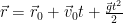
In the project on GitHub1 the particles travel according to Newton’s first law, that is, in straight lines. The trajectory is given by knowing the initial position and velocity by:

If you want to add an external field, let’s say a gravitational one, it is more complicated, but still not a big deal to compute:
In the first case, the velocity doesn’t change until the collision takes place, in the second case it does but it’s also easy to compute:

By the way, if you want, you could change the program to take into account such a field, too.
Here is the code that calculates the position. It uses the Vector3D class already used in the Newtonian gravity program.
1 2 3 4 | inline Vector3D<double> GetPosition(double simTime) const { return position + (simTime - particleTime) * velocity; } |
It’s basically the above formula translated into code (it’s in the Particle class). simTime is the simulation time, particleTime is the time for the ‘initial’ position of the particle. Each particle has its own time, it’s typically the time the particle had a collision but it also can be the time when a particle that had a collision with it scheduled actually collided with another particle (more about this, later).
Location and moment of collision
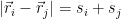
It should be obvious from the above that you must find out only one of them to easily calculate the other one. The condition to have a collision is to have the center of the spheres approaching each other and at the moment of impact the distance between centers is the sum of each ball radius. If we want to calculate the moment of collision for the particles i and j, ignoring for now all the other ones (a particle i can collide with another one before hitting j, but about that, later), we impose the condition of having the distance between them equal with the sum of radii, noted with s here to avoid confusion:
This is a quadratic equation which might have two complex conjugate solutions in which case the ‘particles’ do not collide, or two real solutions. Of course, we are interested only in solutions that are not in the past of any of the involved particles and also the centers should be approaching, not departing. If both solutions are in the future, we pick the first one because the second time is for the case when the particles would depart if they would pass through each other. You’ll find more details about this in the articles, here is the code that deals with the time of collision, also found in the Particle class:
1 2 3 4 5 6 7 8 9 10 11 12 13 14 15 16 17 18 19 20 21 22 23 24 25 26 27 28 29 30 31 32 33 34 35 36 37 38 39 40 41 42 43 44 45 46 47 48 49 50 51 52 53 54 55 | inline double CollisionTime(Particle& other) const { // start from whatever time is bigger, this is the reference time double refTime = std::max<double>(particleTime, other.particleTime); double difTime = other.particleTime - particleTime; Vector3D<double> difPos = position - other.position; // adjust because the particles might not have the same time // there are two cases here: // 1. difTime > 0 means that the 'other' particle time is bigger // refTime is 'other' particle time // in such case 'position' (the position of 'this' particle) must be advanced in time // like this position = position + velocity * difTime // 2. difTime < 0 means that 'this' has the bigger reference time // the position of the 'other' particle must be advanced in time // like this: other.position = other.position + other.velocity * abs(difTime) // in difPos other.position is with '-', difTime is negative so the 'abs' is dropped difPos += (difTime > 0 ? velocity : other.velocity) * difTime; Vector3D<double> difVel = velocity - other.velocity; double b = difPos * difVel; double minDist = radius + other.radius; // collision distance double C = difPos * difPos - minDist * minDist; double difVel2 = difVel * difVel; double delta = b * b - difVel2 * C; // a delta < 0 means to complex solutions, that is, no real solution = the spheres do not collide // delta = 0 is the degenerate case, the spheres meet in the trajectory and depart at the same time = tangential touch, no need to handle it, they are smooth spheres // delta > 0 is the only interesting case // the two different solutions means that there are two times when the spheres are at the radius1 + radius2 distance on their trajectory, which is what we want to consider // the first time is the time they 'meet' and that's the needed time, the time of the collision event after which new velocities must be calculated // the b < 0 condition is the condition that the centers approach, b > 0 means that they are departing if (delta > 0 && b < 0) { double sdelta = sqrt(delta); double t1 = (-b - sdelta) / difVel2; // t2 is not needed, it's the bigger time when they would be again at the radius1+radius2 distance if they would pass through each other //double t2 = (-b + sdelta) / difVel2; // if this time would be negative, that is, it would be as if it took place in the past // perhaps there was a real collision after it that changed the trajectory? if (t1 >= 0) return refTime + t1; } return std::numeric_limits<double>::infinity(); } |
Hopefully the comments are clear enough.
In case you want to add an external field, such as the uniform gravitational field, the trajectories are parabolic. You’ll end up with a quartic equation, which will either have all four roots complex, two roots complex and two real, or all four roots real. In the first case there is no collision, in the second case they would collide only once (there is one real solution for when they meet then the later one for when they would depart if they would pass through one another). In this case the situation is quite similar with the one treated above. With four real roots there are two collisions (and two departures as the ‘particles’ pass through one another). Just pick the first one that is for the future of both particles. I ignored here the degenerate cases, I’ll let the detailed study of roots up to you, if you want to have this coded. Here is a start.
Collision results
The project considers smooth hard spheres. Hard means an infinite potential inside the sphere, and zero outside. The interaction is instantaneous. Smooth means there is no friction between balls, that is, the tangential velocity does not change during the collision. Either of those could be relaxed and modelled in the program, I consider the most interesting one the second one… in that case the state of the ‘particle’ would not be given by only the position and momentum, you will also need the angular momentum. You’ll involve the moment of inertia which for a homogeneous ball of mass m is easy to calculate. Having the balls rotate and change their rotation during the collision would complicate the program quite a bit, but it could be done.
Anyway, the project considers the spheres smooth. Both momentum and kinetic energy are conserved:

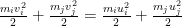
You might think that by writing on vector components you get only four equations but there are six unknowns, but do not forget about the two unchanged tangential components of the velocities. I won’t solve this here, it’s quite easy but I have limited time and I don’t want to type many formulae. If you want to find the solution yourself, you can use the center of mass coordinate system to ease things up. You’ll find out that in that particular coordinate system, the velocities just reverse sign after collision. To turn back to the original coordinate system, just add the velocity of the center of mass to them and that’s it.
Here is the code that calculates the velocities after collision, from the class Simulation:
1 2 3 4 5 6 7 8 9 10 11 | static inline void AdjustVelocitiesForCollision(Particle& particle1, Particle& particle2) { double totalMass = particle1.mass + particle2.mass; Vector3D<double> velDif = particle1.velocity - particle2.velocity; Vector3D<double> dir = (particle1.position - particle2.position).Normalize(); Vector3D<double> mult = 2 * (velDif * dir) * dir / totalMass; particle1.velocity -= particle2.mass * mult; particle2.velocity += particle1.mass * mult; } |
Hopefully I didn’t make a mistake trying to simplify the code.
Walls and other obstacles
I didn’t mention walls when talking about trajectories and collisions above, but the ‘particles’ are contained in a cube. The collisions with the walls are elastic collisions, too. They are quite easy to handle so I’ll let you check out the code for those. Maybe you could add some code for collision with the camera. Just something like a sphere around it with infinite mass. That would provide some nice effects when you move the camera inside the cube. It should be very easy to implement.
Algorithm and possible improvements
Algorithm
Here is the algorithm, presented very shortly:
- Start with initial positions of particles and their velocity. The project for this blog entry just generates positions at random in the cube (taking care to not overlap balls). There are two kinds of ‘particles’, one can specify their mass and radius separately. One kind of particles are generated inside a sphere (also with configurable size) with the center in the center of the cube, the other kind of spheres is generated outside. The speed is the same for all particles, the velocity orientation being random, although one could consider a temperature – or two different ones – instead of a given speed and consider Maxwell-Boltzmann distribution for velocities. This step is implemented in
Simulation::GenerateRandom. - For each N(N-1)/2 pair of particles check if the trajectories allow a collision and if yes, generate a collision event and put it in a priority queue ordered by the collision time.
- Generate a similar event for each of the potential N collisions with the walls. The difference is that the collision event with the wall involves only a particle, instead of two as in the case of two particle collision. The priority queue is built-in
Simulation::BuildEventQueue. - The ‘particles’ move according to the simple rules presented above – either on straight lines or a parabola, until the first collision time.
- The loop of the algorithm starts here: the first collision event is taken out of the even queue. The particles (or particle, for a wall collision event) velocities are updated according to the elastic collision presented above.
- Remove from the events queue all collisions that involve the particle(s) from the current event. They are not going to collide as scheduled because the particle(s) is(are) deviated from the trajectory by the current collision.
- Generate new collision events for the particle(s) involved in the collision – with all the other particles and with walls – and put them in the queue.
- Repeat as necessary.
Basically all the algorithm code is in the Simulation class along with some help from the Particle class. Here is the Advance method:
1 2 3 4 5 6 7 8 9 10 11 12 13 14 15 16 17 18 19 20 21 22 23 24 25 26 27 28 29 30 31 32 33 34 35 36 37 | void Simulation::Advance() { RemoveNoEventsFromQueueFront(); if (eventsQueue.empty()) return; // should not happen, except when there are no particles Event nextEvent = GetAndRemoveFirstEventFromQueue(); int numParticles = (int)particles.size(); AdjustForNextEvent(nextEvent); EraseParticleEventsFromQueue(nextEvent); // also adjusts 'partners' AddWallCollisionToQueue(nextEvent.particle1); if (Event::EventType::particleCollision == nextEvent.type) { AddWallCollisionToQueue(nextEvent.particle2); AddCollision(nextEvent.particle1, nextEvent.particle2); for (int i = 0; i < numParticles; ++i) { if (i != nextEvent.particle1 && i != nextEvent.particle2) { AddCollision(nextEvent.particle1, i); AddCollision(nextEvent.particle2, i); } } } else { for (int i = 0; i < numParticles; ++i) { if (i != nextEvent.particle1) AddCollision(nextEvent.particle1, i); } } } |
For the rest please check out the code on GitHub1.
Improvements
One very important improvement would be to consider periodic boundary conditions. If you don’t want to simulate some very small cavity (or channel, whatever) you would want to have conditions as close as in some bulk liquid or gas, that is, free from surface effects. This can be realized with the periodic boundary conditions. I didn’t implement it because it complicates the code a little bit and it works well together with sectoring, which I also avoided. Please look into the linked articles for details, sectoring increases computation speed even more.
One could extend the program to do other interesting things than diffusion, for example one could add a ‘wall’ that splits the cube that contains the particles in half and allows particles to pass (or be reflected) through it depending on the particle size and mass, perhaps with a probability attached. This would be a model for osmosis. Put a heavy big particle in the middle and simulate Brownian motion. One can think of many other things, especially with an external field added.
How to extract information
There would be many statistics that could be done, as distribution of speeds, collision rate, mean free path, temperature reached when equilibrium is reached (especially if you start out with different temperatures in the beginning as mentioned above) and so on. I won’t give many details, there are some computational physics books I already mentioned on this blog that offer plenty of details on what and how to get information out of molecular dynamics. Maybe I’ll detail this in another post about molecular dynamics.
If I would decide to add some charting to the program, I would probably add one that shows the speed distribution as the system evolves towards equilibrium.
The Code
Especially for the code intended to present some concepts rather than be a production code, I agree with Donald Knuth:
The real problem is that programmers have spent far too much time worrying about efficiency in the wrong places and at the wrong times; premature optimization is the root of all evil (or at least most of it) in programming.
I did not focus on optimization. I tried first to make the code work correctly (although I’m not 100% sure it works all right, I did not test it enough). I consider that the code should first express intent, then one should work on optimization.
At first I simply called the Simulation::Advance from the main thread and it worked quite all right for plenty of particles. The code that does computations should reside in another thread to avoid locking the main thread, so after that I implemented the MolecularDynamicsThread. It uses Advance to generate results that are put in a queue accessed from the main thread. It’s a quite standard producer/consumer code but it still can lock the main thread if the worker thread cannot keep up with the requests, so don’t simulate many particles with a lot of speed. I didn’t think much about it, I just wanted to move out the computation from the main thread. What the main thread gets from the worker thread are ‘snapshots’ of the computation, after each collision. The main thread calculates the actual particle positions using the position, particle time (each particle has its own time) and velocity. Since particles travel in straight lines between collisions, there is no need to move those computations in a separate thread, they are fast enough to not pose problems.
For the same reasons, I used a set::multiset for the events priority queue, although it’s probably implemented with a tree. I did not care about performance at that point. Later, after the first commit on GitHub1, I replaced the multiset with a heap. Since the std priority_queue exposes const iterators, I implemented one myself using std algorithms for a heap. With this change the performance increased a bit. One might do better by looking into heap implementations from boost, but I didn’t consider it necessary for the purpose of the project. The commit has a ‘WARNING!’ in the comment, you might want to get the code with the multiset if you notice bugs in the one with the heap. I turned removing the events from the queue into setting them to ‘no event’ event type instead. Maybe not very elegant, but it works. Those events are removed when they reach to the top of the heap.
OpenGL code
I’ve got the OpenGL code from the Newtonian Gravity project and I customized it to fit this project. First I dropped some classes that are not used, like those for shadow cube map, skybox and textures. I did some copy/paste into the view class for the OpenGL code but there are quite a bit of changes in there. There is also a MolecularDynamicsGLProgram class derived from OpenGL::Program which has quite different shaders compared with the Solar System project. I also changed the OpenGL::Sphere class to allow a useTexture parameter at creation. For this project no texture is used, so it is set to false. There is no need of passing info about texture coordinates if it’s not going to be used. I also added a DrawInstanced method and there is one of the most important change in the OpenGL code compared with the Solar System implementation. In the view you’ll notice that there are three OpenGL::VertexBufferObject, one for color, one for scale and one for position. The scale is set at Setup (for OpenGL) time. In there the color is also set, but that can change later during running. The only thing that changes each frame is the position. The code draws all the spheres by a single call to DrawInstanced after setting the position data all at once in the vertex buffer. I already gave some tutorial links in the Newtonian Mechanics post, I’ll only point to instancing ones now: here8 and here9. It’s not the purpose of this blog to describe in detail OpenGL code so I won’t describe the code more. I’ll mention that I tested it with more than one directional light and it works. Currently it’s a single light only but you can add more in CMolecularDynamicsView::SetupShaders.
Libraries
As for the Solar System project, the program uses mfc, already included with Visual Studio, the obvious OpenGL library and glm10 and glew11.
Classes
I won’t describe here the classes from the OpenGL namespace, I’ll just mention that they are quite thin wrappers around OpenGL API, they typically contain an ID. Please visit the Newtonian Gravity post for more details.
Here it is a short description of the classes, first the ones generated by the App Wizard:
CMolecularDynamicsApp– the application class. There is not much change in there, just added the contained options andInitInstanceis changed to load them and also the registry key is changed toFree App.CMolecularDynamicsDoc– the document class. It contains the data. Since it’s a SDI application, it is reused (that is, it is the same object after you choose ‘New’). There is quite a bit of additions/changes there. It contains the worker thread, the results queue, a mutex that protects the access to the results queue, the ‘simulation time’ and so on. Some of them are atomic for multithreading access although maybe not all that are actually need to be. I did several changes during moving the computation in the worker thread and I probably left some atomic variables that do not need to be.CMolecularDynamicsView– the view class. It take care of displaying. Contains quite a bit of OpenGL code, it deals with key presses and the mouse for camera movements. Among other OpenGL objects it contains the camera, too.CMainFrame– the main frame class. I added there some menu/toolbar handling. It also forwards some mouse and keyboard presses to the view in case it gets them.CAboutDlg– what the name says.
Now, some classes I ‘stole’ from my other open source projects:
CEmbeddedSliderandCMFCToolBarSlider– they implement the slider from the toolbar, used to adjust the simulation speed.CNumberEdit– the edit control for editing double/float values.ComputationThread– the base class for the worker thread.Vector3D– what the name says. First used in the Solar System project. I already anticipated there that I will be using this in other projects.
Classes dealing with options and the UI for them:
Options– the class the contains the options and allows saving them into registry and loading them from registry.COptionsPropertySheet– the property sheet. It’s as generated by the class wizard except that it loads and sets the icon. I already used it in other projects here.SimulationPropertyPage,DisplayPropertyPage,CameraPropertyPage– property pages that are on the property sheet. They are quite standard mfc stuff, I won’t say much about them.
The classes that contain the implementation (apart from the document and the view, you should also check those to understand how it works):
ComputationResult– it’s what the worker thread passes to the main thread. It contains just a list of particles and the next collision time.MolecularDynamicsGLProgram– the OpenGL program. It’s derived fromOpenGL::Programand it deals with shaders, lights and so on.Particle– implements a particle. Contains the particle mass, radius, position and velocity and a ‘particle time’. Has some methods that allows finding out the particle position at a particular time (if it suffers no collision until then), the wall collision time and the collision time with other particle.Event– this implements the events that are in the events queue. The event has a type (currently it can be ‘wall collision’, ‘particles collision’ or ‘no event’), a time of occurrence and it also contains the particles involved. If only a particle is involved, it is set in particle1, the other should be -1.Simulation– as the name says, it is the simulation class. It contains a vector of particles that holds all simulated particles and the events queue, currently implemented with a heap (using a vector container). It has several helper methods, the main one that advances simulation from one collision event to the next one isAdvance.MolecularDynamicsThread– the worker thread. It’s a typical producer/consumer implementation but I feel it’s far from being optimal. My main goal was to have the simulation functional, I didn’t focus on performance, so here it is, something that works. It advances the simulation and it puts the results in the document’s results queue (if not filled up).
Conclusion
That’s about it. Unfortunately I didn’t have time for more details but I guess this is more than nothing.
If you notice and mistakes/bugs or if you have some improvements, please point them out in a comment.
- EventMolecularDynamics The project on GitHub. ↩ ↩ ↩ ↩
- Studies in Molecular Dynamics by B. J. Alder and T. E. Wainwright ↩
- Achieving O(N) in simulating the billiards problem in discrete-event simulation by Gary Harless ↩
- Stable algorithm for event detection in event-driven particle dynamics by Marcus N. Bannerman, Severin Strobl, Arno Formella and Thorsten Poschel ↩
- How to Simulate Billiards and Similar Systems by Boris D. Lubachevsky ↩
- Packing hyperspheres in high-dimensional Euclidean spaces by Monica Skoge, Aleksandar Donev, Frank H. Stillinger, and Salvatore Torquato ↩
- Parallel Discrete Event Simulation of Molecular Dynamics Through Event-Based Decomposition by Martin C. Herbordt, Md. Ashfaquzzaman Khan and Tony Dean ↩
- Instancing on ‘Learn OpenGL’ ↩
- Particles/Instancing on opengl-tutorial.org. ↩
- OpenGL Mathematics ↩
- The OpenGL Extension Wrangler Library ↩

You are a life saver sir. Nicely written. Wanted to see more. Will you implement Time driven method i.e., Discrete element method
Maybe on another subject, definitively not for smooth hard balls, the time driven method is useful when the interaction has a ‘long’ range. You might want to check the Newtonian Gravity post for such an application.
The only problem I see with the whole overly-complex code, is the fact that it defeats the original intent of the goal, and fails in detecting collisions correctly, at all. Don’t let that observation discourage you, it is freaking awesome, what you have setup to work.
The original intent was to limit thinking about objects that are not near colliding, while “accurately” detecting active collisions, for accurate calculations. Though you may be spending less time looking at non-collisions, you also seem to be spending as much time not looking at potential collisions. (I can visually see balls inside one of another and “sticking” together. That is a sign that the collision was not correctly detected, nor was the collision value correctly calculated. (Even if the balls merged, the correct collision would not be linear “sticking” travel. Thus, the calculation itself is incorrect, as well as the merged spheres.)
When texting, do not test a “flock”, until you have tested specific isolated instances… Launch one ball at another, head-on, and at various angles and speeds. When you have correctly seen 0-360 degree intersections with two spheres, try three, then four, then five…
Once those steps have passed, then throw thousands into a box and test it, but give them some room to move, and add some form of gravity, so it eventually ends where you can see the slow-velocity “stacking”, as you slice through the layers of balls, looking for failed collisions. (With the ability to step-into and step-out-of the sequence of animations, to see where it fails, and the corresponding values for the two failed balls.
If by ‘I can visually see balls inside one of another and “sticking” together’ you mean in the video above, indeed I think it had a bug that could allow that. If you mean the latest code, it would be great if you could indicate a way to reproduce it. I did try the code with only a few balls, by the way. It did not exhibit the behavior you claim, but indeed I did not test it a lot.
Even in the video above, it could be great if you could indicate the time position and the approximate place where you’ve seen that.
PS Since the author of the comment above did not bother to detail what he claimed to notice, his comment will be an example in ‘About this blog’ in a future section about comments. A negative one.
Here is a video with only a few balls.
https://www.youtube.com/watch?v=K9z132yiqkY
As usual, it’s jerky because of the screen recording app. The things one should take into account when testing:
– collision with the walls has a good chance to be ok, if not when simulating thousands of balls they could easily escape out and due of their number it would happen rather quickly.
– it’s a 3D simulation. That means that balls can pass behind one another and one can ‘visually see’ them as passing through one another when they are not. The same might happen with ‘sticking’. The perspective can fool you. It’s not always what you ‘see’. Be aware that they are in a cube with invisible walls. That is, you don’t ‘see’ them. That can visually fool you, too.
– the red balls can have not only the different size compared with the green ones, but also different mass. People tend to have a very bad intuition of what should happen in an elastic collision between such balls. youtube is full of people of different weights that are running at one another with big air filled balls in front of them, to check what happens when they collide. Many do not expect the outcome.
– in the video from this comment, at the end the balls are quite tightly packed. In such case because there are many collisions, the balls are quite big while the space between them is small, sticking and passing through should manifest rather easily (not the kind described at the end, that could happen, too, but it’s another matter).
– if you think you found a bug or some error in the description, be more specific. If you have a problem with the theory in the linked articles, say so, I’ll decide you are a troll and you’ll have no more comments here like that 🙂 You’ll have to publish instead and be able to wipe out quite a bit of molecular dynamics simulations.
– I agree I was rushing to post this, I had to leave the country and I wanted to post it before that. I can do mistakes and that’s one reason why I also link to other sources of information. Be aware that this is open source software, it can have bugs as I already specified on the ‘About this blog’ page. If you find such bugs, be specific. ‘I can see’ is not specific. It might mean you are under some hallucinogenic influence, for example. You may point out the problem in the algorithm description above. It might be just a problem with the description, or also with the implementation. If you are able to explain why it fails, please do so. I will try to fix it.
– asking me to add gravitation when I specifically said I won’t is rather odd. I explained how it should be done, for now I don’t intend to complicate the code more. After you complain that the code is overly-complex, asking for having it more so is odd indeed. Maybe you want me to add sectoring, too and then have more reasons to complain?
Now, there is one way of having the balls pass through one another or escape from the cube: by having the worker thread work hard and not be able to supply on time the next collision setup. The main thread will continue to extrapolate from what it has and balls will continue their straight paths through each other or through walls. This is by design and I don’t consider it a bug. When the next state is available the positions will ‘reset’. The alternative was to ‘freeze’ the frame until the worker thread gives more data and I simply didn’t want to do that.