
Introduction
The first post on this blog dealt with Newtonian mechanics, it seems natural to follow it with another big name in physics and another important field. So here it is, something linked to Maxwell and with his equations. Something still simple for now, a program to visualize the electric field in 2D. Here is a video of the program in action:
Here1 is the project. The program is simpler because there is no OpenGL. The numerical methods might be a little more difficult, though. Also there is some more multithreading involved. The program presented is one of the few cases where the Euler method would be ok, it does not need much precision since it’s only for visualization purposes. I implemented Runge-Kutta instead – it includes Euler as a particular case, though – to present more numerical methods and to have something for later, hopefully I’ll reuse the code. Otherwise the implemented numerical methods (except Euler and perhaps midpoint) are overkill. This project was also an opportunity for some tests on the methods I implemented.
The Physics
For such a simple application, one could start with Coulomb’s law and a simple definition for the potential. That would be enough. A quick look at Maxwell equations shouldn’t hurt, either. They are also on the header picture of this blog, on the right. This is electrostatics, so we can drop anything that has a time derivative in there, electric current and obviously, magnetic field. We end up with Gauss law:

By applying Gauss theorem it can be written in integral form:

where Q is the total charge in the volume V, S is the surface around the volume V. 


The electric field for such a charge is easy to calculate:

where r is the distance from the center of the sphere. One can easily see where the 


The field from such a charge is easy to calculate in the code, so here it is, from the class Charge:
1 2 3 4 5 6 7 8 9 10 | inline Vector2D<double> E(const Vector2D<double>& pos) const { Vector2D<double> toPos = pos - position; double len2 = toPos * toPos; Vector2D<double> result = toPos / (len2 * sqrt(len2)); result *= charge; return result; } |
As you can notice, I prefer to drop out constants from the calculations, they are not relevant. position is the position of the charge.
As for the gravitational field, superposition works:

that is, to calculate the electric field in a point, one simply adds all fields generated by each charge (for a charge distribution the sum becomes an integral). It’s quite easy to do in the code, so here it is, from the class TheElectricField:
1 2 3 4 5 6 7 8 9 | inline Vector2D<double> E(const Vector2D<double>& pos) const { Vector2D<double> result; for (auto &&charge : charges) result += charge.E(pos); return result; } |
Using 


Charge:
1 2 3 4 | inline double Potential(const Vector2D<double>& pos) const { return charge / (pos - position).Length(); } |
and the potential for all charges from the class TheElectricField:
1 2 3 4 5 6 7 8 9 | inline double Potential(const Vector2D<double>& pos) const { double P = 0; for (auto &&charge : charges) P += charge.Potential(pos); return P; } |
Just to end this theoretical part, this particular situation is called electrostatics, but it’s still electromagnetism. If you want to see where the ‘magnetism’ part is, imagine that you are in a particular reference frame when you are looking at the charges. The Universe does not really care about what reference frame did you pick. The situation might look different to you, but the physics is the same, it’s not dependent on how you look at it. Now look at the charges from a reference frame that is moving relative to them. Moving charges means an electric current, an electric current means a magnetic field. So there it is, the magnetism part is hidden because of your perspective. There is no such thing as a separate electric field and a separate magnetic field. They are part of the same field, the electromagnetic field.
Field Lines
Field lines are an useful tool for visualizing vector fields. In our 2D case we have two kinds of lines, the electric field lines and the equipotentials. The later are actually surfaces in 3D. The electric field lines have the electric field vector as a tangent and their density is proportional with the magnitude of the electric field. This already poses a problem in a 2D representation, because their density for a point charge in the 2D representation drops as 
Since I mentioned a problem, I should mention another one until I forget. Field lines start on sources and end on sinks. Their number, for equal size spheres that contain the spherically symmetrical distributed charge, is proportional with the charge. But that is true for spheres, that is, in 3D. For 2D we have circles instead but the code still starts twice as many lines from a charge with the value 2 than from one with the value 1 (should do that by distributing them on the whole surface of the sphere instead). I wouldn’t like to have a non integer number of lines, if you know what I mean… that’s also a reason why I allow only integer values for charges. If not integer, it would also rise some issues with the potential.
Despite this, the code still is ok if you keep that in mind. That’s why it says on titles ‘unequal charges’ without specifying the ratio between them. The only place where it might confuse is the options, but since you are warned now, it should be all right. One should be able to calculate the ‘true’ charge knowing the values for the area of the sphere versus the circumference of the circle.
So, the field line is given by the direction of the vector. That already suggests using the Euler method: just calculate the electric field in the start point, jump a step in its direction, repeat again and again for the current point until either it reaches a sink or it’s long enough that there is no hope returning on a charge. There are simplifications to this, for example if all charges have the same sign, you already know that the field lines won’t return, but about those, later. But, is it ok to jump the same step size from different points, no matter if the line is almost straight or it bends quite a bit? It looks like even this would benefit from higher order methods and why not, even from adaptive methods.
Before going into the actual numerical methods, let’s see how it would be solved with Euler (which, again, will be a particular case). We would have 

That means it’s not really a function (not in the usual sense, for more see multivalued function). You might try to parametrize the curve stating that 


Then 
Can we do better and clearly? With a little bit of geometrical thinking, yes we can. First, let’s drop the coordinate system and think in terms of vectors. They are mathematical objects that do not depend on coordinates. Imagine our field line. In a certain point on it the infinitesimal vector along the curve is 


That’s it. We have enough to use the numerical algorithms to find the field line.
The algorithms can be used to solve problems where one has the initial conditions and knows the “time” derivative of a function 
In our case, “time” t is not really time, but the position on the line given by the line length, measured from the start. One could think of it as time if he imagines a small charge travelling along the line. The picture is not entirely physical, because the presence of another charge changes the configuration of the field and besides, it has mass. From the previous post one can notice that things with mass do not necessarily travel in the direction the field tells them to. One still could imagine various setups where the approximation is good enough (very small mass, in a fluid that has drag forcing it to move with a small speed and so on). In a sense, it is time (for the non adaptive methods). It’s the time needed for the calculation to reach that point. But that’s less physical than the travel distance.
No matter how you look at it, you might notice that you don’t really need the “time” for this case, the function is less general.
The function is now quite clear for the electric field lines, but how about equipotentials? You want to draw the line through points that have the same potential, that is, a constant potential. That means a zero directional derivative. That means it is orthogonal on the direction of the maximum directional derivative in that point, that is the gradient, but that’s how the potential is linked to the electric field. So one can use a function that is very similar with that for the electric field line, the vector just needs to be rotated with 
Here are the needed functions implemented in the program (in the ComputationThread class which is defined in the FieldLinesCalculator class):
1 2 3 4 5 6 7 8 9 10 11 12 13 14 15 16 17 18 19 20 21 22 23 24 25 26 27 28 29 30 31 32 33 34 35 | class FunctorForCalc { public: const TheElectricField *theField; FunctorForCalc(const TheElectricField *field = NULL) : theField(field) {} }; class FunctorForE : public FunctorForCalc { public: int charge_sign; FunctorForE(const TheElectricField *field = NULL) : FunctorForCalc(field), charge_sign(1) {}; inline Vector2D<double> operator()(double /*t*/, const Vector2D<double>& pos) { Vector2D<double> v = theField->ENormalized(pos); return charge_sign > 0 ? v : -v; }; }; class FunctorForV : public FunctorForCalc { public: FunctorForV(const TheElectricField *field = NULL) : FunctorForCalc(field) {}; // just returns a perpendicular vector on E inline Vector2D<double> operator()(double /*t*/, const Vector2D<double>& pos) { Vector2D<double> v = theField->E(pos); double temp = v.X; v.X = -v.Y; v.Y = temp; return v.Normalize(); }; }; |
They do not need much explanations, the functor for E changes sign for negative charges because you don’t want to go along a line towards the charge center, you want the line to go from the charge, outside. Odd things would happen if the line would reach the center, because the code considers point charges. That means a singularity in the center, that is, an infinite field because of the division with 
Numerical Methods
The numerical methods used are the Runge-Kutta methods, more specifically, the explicit ones, including adaptive methods. Before trying to understand them, please be sure to understand the Euler method and the midpoint method, they are particular cases of Runge-Kutta methods and they are easy to understand.
The general Runge-Kutta method is expressed as:
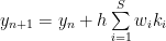
where

S is the number of stages of the particular Runge-Kutta method, i is the current stage during calculations, the 


The simplest Runge-Kutta method is the Euler method. It has a single stage, the node is at the current position and the weight is 1, that is the slope estimated at 


From the ones with two stages, second order methods, I implemented the midpoint, Heun and Ralston methods. The midpoint method has nodes at the current “time” and at the next “time” instant (that is, the node values are 0 and 1) but the weight is zero for the first slope estimation and 1 for the next (and last) one. The end result is that the midpoint method advances by using a slope calculated in a point obtained by advancing half a step using the slope in the current point. The slope is evaluated for a value of half the time step, too. As a formula, the slope used is 
The Heun method (also called improved Euler) evaluates the slope by averaging two slope values, one obtained at the current position and one by advancing one step (both “time” and “space”), using the first evaluated slope. That means that the two weights are 1/2 each. The nodes are at 0 and 1. The Ralston method is similar, but its weights are 1/4 and 3/4, that is the slope evaluated after advancing is given more weight than for the slope at the current point. The nodes are at 0 and 2/3, so it does not try to advance a full step ahead to evaluate the slope, but only 2/3 of it (the a coefficient is also 2/3).
After understanding the above methods, the RK4 method should be easy to understand, too. It’s a fourth order method, with four slope estimations. The ones estimated for the current point and for the one after a time step (nodes with the values 0 and 1) are given half the weight for the estimations between them (nodes with value 1/2). It should be easy to understand because there is only one non zero a coefficient on each tableau line, that is, only the slope estimation from the previous stage is used in the current stage (to advance at a point for the next slope estimation). The more complicated ones use a weighted average of the previously estimated slopes.
For more information, please visit the links I provided, they are way more detailed (including a proof using Taylor expansion). Here is the code that implements the Runge-Kutta methods:
1 2 3 4 5 6 7 8 9 10 11 12 13 14 15 16 17 18 19 20 21 22 23 24 25 26 27 28 29 30 31 32 33 | template<typename T, unsigned int Stages> class RungeKutta { protected: std::array<double, Stages> m_weights; std::array<double, Stages> m_nodes; std::vector<std::vector<double>> m_coefficients; std::array<T, Stages> K; public: RungeKutta(const double weights[], const double nodes[], const double *coefficients[]); template<typename Func> inline T SolveStep(Func& Function, const T& curVal, double t, double h) { T thesum(0); for (unsigned int stage = 0; stage < Stages; ++stage) { T accum(0); for (unsigned int j = 0; j < stage; ++j) accum += m_coefficients[stage - 1][j] * K[j]; K[stage] = Function(t + m_nodes[stage] * h, curVal + h * accum); thesum += m_weights[stage] * K[stage]; } return curVal + h * thesum; } template<typename Func> inline T SolveStep(Func& Function, const T& curVal, double t, double& h, double& /*next_h*/, double /*tolerance*/, double /*max_step*/ = DBL_MAX, double /*min_step*/ = DBL_MIN) { //next_h = h; return SolveStep(Function, curVal, t, h); } bool IsAdaptive() const { return false; } }; |
A particular Runge-Kutta method is implemented by deriving from this class, it’s very easy:
1 2 3 4 5 | template<typename T> class RK4 : public RungeKutta<T, 4> { public: RK4(void); }; |
The constructor just sets the tableau and that’s about it:
1 2 3 4 5 6 7 8 9 10 11 12 | static const double RK4weights[] = { 1. / 6., 1. / 3., 1. / 3., 1. / 6. }; static const double RK4nodes[] = { 0, 1. / 2., 1. / 2., 1. }; static const double row1[] = { 1. / 2. }; static const double row2[] = { 0, 1. / 2. }; static const double row3[] = { 0, 0, 1 }; static const double *RK4coeff[] = { row1, row2, row3 }; template<typename T> RK4<T>::RK4(void) : RungeKutta(RK4weights, RK4nodes, RK4coeff) { } |
I also implemented adaptive methods, but for the code for them you’ll have to look into the sources1. AdaptiveRungeKutta is derived from the RungeKutta class and from it all adaptive methods are derived. Very shortly, there is another row of weights that allows calculating (looping over stages only once) instead of a single result, two estimations, one with a higher order (with 1) than the other. This allows to estimate the error by pretending that the higher order result is exact and claiming that the difference among them is the error. This difference allows adjusting the step to reach a higher precision (the desired precision can be specified). The adjustment is done by taking into account the order. The adaptive methods have a variable step size. Please look in the code for implementation, the method should be quite clear. It resembles the RungeKutta implementations, there is just one more for loop for step size adjustment, each stage two values are computed (see thesumLow and thesumHigh values) and most of the code that is different (supplementary) deals with adjusting the step.
To present an example on how such algoritm is used, here is the method that calculates the equipotential line:
1 2 3 4 5 6 7 8 9 10 11 12 13 14 15 16 17 18 19 20 21 22 23 24 25 26 27 28 29 30 31 32 33 34 35 36 37 38 | template<class T> inline void FieldLinesCalculator::CalcThread<T>::CalculateEquipotential() { Vector2D<double> startPoint = m_Job.point; Vector2D<double> point = startPoint; double dist = 0; double t = 0; unsigned int num_steps = (m_Solver->IsAdaptive() ? 800000 : 1500000); double step = (m_Solver->IsAdaptive() ? 0.001 : 0.0001); double next_step = step; fieldLine.AddPoint(startPoint); fieldLine.weightCenter = Vector2D<double>(startPoint); for (unsigned int i = 0; i < num_steps; ++i) { point = m_Solver->SolveStep(functorV, point, t, step, next_step, 1E-3, 0.01); fieldLine.AddPoint(point); // 'step' plays the role of the portion of the curve 'weight' fieldLine.weightCenter += point * step; t += step; if (m_Solver->IsAdaptive()) step = next_step; // if the distance is smaller than 6 logical units but the line length is bigger than // double the distance from the start point // the code assumes that the field line closes dist = (startPoint - point).Length(); if (dist * distanceUnitLength < 6. && t > 2.*dist) { fieldLine.points.push_back(startPoint); // close the loop fieldLine.weightCenter /= t; // divide by the whole 'weight' of the curve break; } } } |
The one that calculates the electric field line is quite similar, but a little bit longer because there are more checks in there. I added comments in both of them that should help understanding the intent of the code. If you are curious what weightCenter is and does in the code above, it is just that, a weight center for the equipotential loop. I use it to remove some duplicates of the equipotential lines. They are calculated starting from the first electric line from each charge and that creates duplicates which are removed at the end of the calculations. More details about that, later. AddPoint does not really add each point to the line, but only those that are far enough from the previous one. ‘Far enough’ depends on how close they are from the start of the line. Obviously one does not need a lot of points to represent a portion of line that’s off the screen and does not curve so much there.
To be noted that the Runge-Kutta implementation might be quite far from the performance one could achieve by coding a particular method. A good compiler might unroll the loops and take advantage by the knowledge of the tableau at compile time to optimize calculations, for example avoiding unnecessary multiplications where the terms are zero and the additions of zero values, but one might achieve better performance by coding and optimizing a particular method only. As a warning, if you use it in your code, please check the code and the Butcher tableau values, I offer no warranty that they are correct.
The Code
Drawing
The program uses Direct2D for drawing in the view, but GDI for printing and print preview drawing. The reason is the mfc print preview implementation. I didn’t want to look into the mfc code to see if I could change the print preview to be able to draw with Direct2D, so I preferred to expose a pair of Draw methods, one that draws with Direct2D and one that uses GDI (not GDI+, I’ll use that in future projects posted here, though). Although the drawing methods are quite similar, there are differences enforced by library limitations. For example GDI ability to draw Bezier curves is quite limited, one cannot add as many points as he would like to a call to PolyBezier, while a Direct2D path is more capable. Please see the code1 for details (FieldLine::Draw methods specifically).
As typical in mfc programs, the view draws itself. After preparing the rendering target, the view asks the field object to draw itself, which in turn delegates drawing to charges and field lines objects:
1 2 3 4 5 6 7 8 9 10 11 12 13 14 | void TheElectricField::Draw(CHwndRenderTarget* renderTarget, CRect& rect) { // draw electric field lines for (auto &&line : electricFieldLines) line.Draw(renderTarget, rect); // draw potential lines for (auto &&line : potentialFieldLines) line.Draw(renderTarget, rect, true); // draw charges for (auto &&charge : charges) charge.Draw(renderTarget, rect); } |
For the other drawing methods please check the code1, they should be quite clear.
Bézier and Spline curves
An easy option for drawing the field lines would be simply to draw line segments between the points. That obviously does not look so good, especially if you space the points at bigger distance. A nicer look would be given by a Spline curve but unfortunately I couldn’t find an implementation in Direct2D – although GDI+ has one – so I had to use Bézier curves instead, more specifically, cubic ones. Since points are not so far apart and field lines are well behaved, it doesn’t make much difference visually, although it wouldn’t be exactly correct. That bothered me a little so I took a pen and paper and with not much more explanation, here is the result:
1 2 3 4 5 6 7 8 9 10 11 12 13 14 15 16 17 18 19 20 21 22 23 24 25 | void FieldLine::AdjustForBezier(const Vector2D<double>& pt0, const Vector2D<double>& pt1, const Vector2D<double>& pt2, const Vector2D<double>& pt3, double& Xo1, double& Yo1, double& Xo2, double& Yo2) { double t1 = (pt1 - pt0).Length(); double t2 = t1 + (pt2 - pt1).Length(); double t3 = t1 + t2 + (pt3 - pt2).Length(); t1 /= t3; t2 /= t3; double divi = 3. * t1 * t2 * (1. - t1) * (1. - t2) * (t2 - t1); ASSERT(abs(divi) > DBL_MIN); double a = t2 * (1. - t2) * (pt1.X - (1. - t1) * (1. - t1) * (1. - t1) * pt0.X - t1 * t1 * t1 * pt3.X); double b = t1 * (1. - t1) * (pt2.X - (1. - t2) * (1. - t2) * (1. - t2) * pt0.X - t2 * t2 * t2 * pt3.X); Xo1 = (t2 * a - t1 * b) / divi; Xo2 = ((1. - t1) * b - (1. - t2) * a) / divi; a = t2 * (1. - t2) * (pt1.Y - (1. - t1) * (1. - t1) * (1. - t1) * pt0.Y - t1 * t1 * t1 * pt3.Y); b = t1 * (1. - t1) * (pt2.Y - (1. - t2) * (1. - t2) * (1. - t2) * pt0.Y - t2 * t2 * t2 * pt3.Y); Yo1 = (t2 * a - t1 * b) / divi; Yo2 = ((1. - t1) * b - (1. - t2) * a) / divi; } |
The code adjusts the intermediate points (control points) in such a way that the new control points make the curve pass through the original points. Obviously it is not enough to have the original four points you want the curve to pass through to get the Bézier curve, there are an infinity of such curves passing through all four points. One more condition is required, and that’s the (relative) length of each curve segment. The Wikipedia page mentions a special case – where one gets nicer formulae – when t=1/3 and t=2/3 for the position of the intermediary points, here it is more general. I chose to approximate the length with the distance between points, in this particular case one could do even better, by using the field line lengths as calculated during field line computation… but this should be good enough, I didn’t want to complicate the code that much.
Multithreading
Unlike the case for the previous post, where only a single computing thread was used, this program deals with multithreading much more.
There is code that simply splits work into two threads like this – in CElectricFieldDoc::GetData():
1 2 3 4 5 | std::thread thread1 = std::thread([calc = calculator] { for (auto& line : calc->field.electricFieldLines) line.AdjustForBezier(); }); std::thread thread2 = std::thread([calc = calculator] { for (auto& line : calc->field.potentialFieldLines) line.AdjustForBezier(); }); thread1.join(); thread2.join(); |
This code would benefit from splitting the code between more threads and not joining them, like the case for the field lines, but not so much so I did not bother. It’s more clear this way, much complex code wouldn’t help that much.
The code for calculating the field lines is able to split the work among many threads, their number being configurable. In order to do that, I implemented a queue of ‘jobs’ (like this: std::deque<FieldLineJob> m_jobs;) and I started a pool of threads that take jobs from there and execute them. Here is the code that makes the initial ‘jobs’ and starts the threads:
1 2 3 4 5 6 7 8 9 10 11 12 13 14 15 16 17 18 19 20 21 22 23 24 25 26 27 28 29 30 31 32 33 34 35 36 37 38 | void FieldLinesCalculator::StartCalculating(const TheElectricField *theField) { Clear(); if (NULL == theField) return; bool has_different_signs; int total_charge = theField->GetTotalCharge(has_different_signs); Vector2D<double> point; double angle_start = 0; for (auto &&charge : theField->charges) { if (charge.charge == 0) continue; double angle_step = 2.*M_PI / (fabs(charge.charge)*theApp.options.numLinesOnUnitCharge); angle_start = - angle_step / 2. - M_PI; if (sign(total_charge) != sign(charge.charge)) angle_start += M_PI + angle_step; for (double angle = angle_start; angle < 2.*M_PI + angle_start - angle_step / 4.; angle += angle_step) { if ((angle != angle_start || !theApp.options.calculateEquipotentials) && sign(total_charge) != sign(charge.charge)) break; double r = theApp.options.chargeRadius / theApp.options.distanceUnitLength; point.X = charge.position.X + r*cos(angle); point.Y = charge.position.Y + r*sin(angle); m_jobs.push_back( { charge, total_charge, has_different_signs, angle, angle_start, point, false, 0 } ); } } potentialInterval = theApp.options.potentialInterval; calcMethod = theApp.options.calculationMethod; startedThreads = theApp.options.numThreads; for (unsigned int i = 0; i < startedThreads; ++i) StartComputingThread(theField); } |
It should be easy to understand: the code just walks around the charges making ‘jobs’ by setting the initial position of the field line and some info needed during calculation, then it starts the threads.
A thread has its loop implemented like this:
1 2 3 4 5 6 7 8 9 10 11 12 13 14 15 16 17 18 19 20 21 22 23 24 25 26 27 28 29 30 31 32 33 34 35 36 37 38 39 40 41 42 43 44 | template<class T> void FieldLinesCalculator::CalcThread<T>::Calculate() { for (;;) { // grab a job from the job list { std::lock_guard<std::mutex> lock(m_pCalculator->m_jobsSection); if (m_pCalculator->Terminate || m_pCalculator->m_jobs.empty()) break; // no more jobs or asked to finish m_Job = m_pCalculator->m_jobs.front(); m_pCalculator->m_jobs.pop_front(); } if (m_Job.isEquipotential) { CalculateEquipotential(); if (m_pCalculator->Terminate) break; std::lock_guard<std::mutex> lock(m_pCalculator->m_potentialLinesSection); m_pCalculator->potentialFieldLines.push_back(PotentialLine()); m_pCalculator->potentialFieldLines.back().potential = m_Job.old_potential; m_pCalculator->potentialFieldLines.back().weightCenter = fieldLine.weightCenter; m_pCalculator->potentialFieldLines.back().points.swap(fieldLine.points); } else { functorE.charge_sign = sign(m_Job.charge.charge); CalculateElectricFieldLine(); if (m_pCalculator->Terminate) break; std::lock_guard<std::mutex> lock(m_pCalculator->m_electricLinesSection); m_pCalculator->electricFieldLines.push_back(FieldLine()); m_pCalculator->electricFieldLines.back().points.swap(fieldLine.points); } } FieldLinesCalculator* calc = m_pCalculator; delete this; ++calc->finishedThreads; } |
Again it should be quite straightforward: the thread continues to take out jobs until there are no jobs left. Depending on the type of job, it calculates either an equipotential line or an electric field line.
The first electric field line computation is also responsible for posting equipotential jobs:
1 2 3 4 5 6 7 8 9 10 11 12 13 14 15 16 17 18 19 20 21 22 23 24 25 26 27 | template<class T> inline void FieldLinesCalculator::CalcThread<T>::PostCalculateEquipotential() { if (m_Job.angle != m_Job.angle_start || !calculateEquipotentials) return; Vector2D<double> startPoint = m_Job.point; double potential = functorV.theField->Potential(startPoint); if (sign(m_Job.charge.charge)*sign(potential) > 0 && abs(m_Job.old_potential - potential) >= potentialInterval) { if (m_Job.old_potential == 0) m_Job.old_potential = floor(potential / potentialInterval) * potentialInterval; else m_Job.old_potential += sign(potential - m_Job.old_potential) * potentialInterval; std::lock_guard<std::mutex> lock(m_pCalculator->m_jobsSection); FieldLineJob job(m_Job); job.isEquipotential = true; m_pCalculator->m_jobs.push_back(job); // some threads finished although there are still jobs posted // restart one if (m_pCalculator->finishedThreads > 0) { --m_pCalculator->finishedThreads; m_pCalculator->StartComputingThread(&m_pCalculator->field); } } } |
It might be the case that the computation threads exhausted the jobs queue before another job is posted and some of them ended, so the code restarts a thread if that’s the case.
There is a timer set in the view that checks from time to time for threads termination. If they all ended, the data is retrieved and adjusted, before drawing. One adjustment is for Bézier lines, the other one deals with removing the duplicates from equipotential lines.
Removing equipotential duplicates
The reason why duplicates arise is that equipotential lines are calculated starting from an electric field line that originates from each charge (one for each charge). One gets lines that are at the same potential but go around different charges, so they don’t coincide, but in other cases they go around more than one charge and duplicates occur. To remove them I wrote some code that is neither clean, nor efficient (it even runs in the main thread) but at the time I wrote it I was quite bored by the project and wanted to finish it. You’ll find that code in void CElectricFieldDoc::GetDataFromThreads(). It uses a ‘weight center’ for the equipotential line to decide if different lines are for the same equipotential line or not. The code first sorts the lines in the potential order to separate them by the potential value, then it distinguishes them further using that ‘weight center’. Two points with about the same weight center – having about the same potential, too – are considered the same. I used the distance from an arbitrary point to the weight center to sort them, so the code could be fooled, but in practice it is good enough for the purpose of the project.
Classes
Here is a short description of the classes in the project, also available in the README file:
First, the classes generated by the MFC Application Wizard:
CAboutDlg – What the name says, I don’t think it needs more explanation.
CChildFrame – It’s a MDI application, this is the child frame. No change done to the generated class.
CMainFrame – Just a little bit of change to the generated one. The main one is the addition of the OnViewOptions() handler which displays the options property page.
CElectricFieldDoc – The document. Contains the ‘field lines calculator’ object. It’s the base class for derived documents which implement particular charge configurations. Has a couple of GetData methods that deal with data retrieval and adjustment from the calculator and a CheckStatus that forwards the call to the calculator object, to check if the computing threads finished. The OnCloseDocument method called when a document is closed checks to see if threads were finished. If yes, the calculator object is deleted, if not, it is moved in the application object – after asking the threads for termination – where it stays until the threads are finished.
CElectricFieldView – The view class. It is changed to use Direct2D for displaying, except print preview and printing where it still uses gdi. The drawing is delegated to charges and field lines objects through the field object that is contained in the calculator (contained in the document). Has a timer set that allows checking for field lines data availability in the document.
CElectricFieldApp – The application class. Has minor changes and lots of document templates additions, one for each charge configuration from the program. Has a vector of ‘calculators’ that contains calculator objects from the documents that were closed before the threads finished. ExitInstance calls OnIdle until all threads are finished. OnIdle removes and deletes the calculator objects which have the computing threads finished.
The classes that deal with settings:
Options – This is the settings class. Load loads them from the registry, Save writes them into registry.
OptionsPropertySheet, ComputationPropertyPage, DrawPropertyPage – UI for the options. Not a big deal, should be easy to understand.
PrecisionTimer is a class that I used to measure some execution times. Not currently used in the program, it might be useful in some other projects, too.
Vector2D<T> – It’s very similar with the Vector3D
ComputationThread – The base class for a field line computation thread. There is not much to it, Start() starts it.
FieldLinesCalculator – Contains the field object, the jobs queue, data from calculating threads, deals with the computing threads.
FieldLinesCalculator::CalcThread – The computing thread. Calculates electric field lines and equipotentials. Also posts equipotential jobs if it’s the first electric field line/charge that it’s calculating.
TheElectricField – The electric field class. Contains the charges and the electric field lines and equipotentials. Has methods to calculate the electric field and the potential and some other helper ones. Can draw itself by asking each charge and line to draw itself.
Charge – The charge class, has ‘charge’ and ‘position’. Can draw itself and also can calculate the electric field and potential due of the charge it represents.
FieldLine – A field line. Instances of it are electric field lines. Contains the points and it has drawing methods and the Bezier adjustment code.
PotentialLine – Derived from the above to just contain the potential and the weight center.
The RungeKutta namespace contains the Runge-Kutta methods classes.
RungeKutta<T, Stages> – It is the base class, implements Runge-Kutta. The methods are derived from it.
AdaptiveRungeKutta<T, Stages, Order> – Adaptive Runge-Kutta. The adaptive methods are derived from it.
For the other ones, please see the code.
The ChargeConfiguration namespace contains classes derived from the document. They implement the particular charge configurations.
Adding Charges Configurations
I didn’t want to implement loading the document from an xml file, for how to do that please see the previous post. I took advantage of the mfc document template and hardwired the charges configuration in the program instead. Here is how one could extend them:
The first step would be to derive a class from CElectricFieldDoc. I put them all in the ChargeConfiguration namespace.
1 2 3 4 5 | class CDipoleDoc : public CElectricFieldDoc { DECLARE_DYNCREATE(CDipoleDoc) public: virtual BOOL OnNewDocument(); }; |
Only OnNewDocument must be overridden. In there one adds the charges and then the calculation is started and that’s about it.
1 2 3 4 5 6 7 8 9 10 11 12 13 14 15 16 17 18 19 20 21 22 23 24 25 | IMPLEMENT_DYNCREATE(CDipoleDoc, CElectricFieldDoc) BOOL CDipoleDoc::OnNewDocument() { if (!CElectricFieldDoc::OnNewDocument()) return FALSE; // TODO: add reinitialization code here // (SDI documents will reuse this document) Charge charge; charge.position = Vector2D<double>(-2, 0); charge.charge = 1; calculator->field.charges.push_back(charge); charge.charge = -1; charge.position = Vector2D<double>(2, 0); calculator->field.charges.push_back(charge); calculator->StartCalculating(&calculator->field); return TRUE; } |
The second step is to add the document template in CElectricFieldApp::InitInstance().
1 2 3 4 5 6 7 8 | CMultiDocTemplate* pDocTemplate; pDocTemplate = new CMultiDocTemplate(IDR_DipoleTYPE, RUNTIME_CLASS(CDipoleDoc), RUNTIME_CLASS(CChildFrame), // custom MDI child frame RUNTIME_CLASS(CElectricFieldView)); if (!pDocTemplate) return FALSE; AddDocTemplate(pDocTemplate); |
The third step would be to add corresponding resources, string resource for names (as in IDR_DipoleTYPE \nDipole\nDipole\n\n\n\n), the menu resource (just copy the dipole one and change the id to whatever IDR_ you use) and icon. Be sure that the IDR_ id matches the one used for the document template.
Conclusion
This program is far from being perfect, I even mentioned in the text how it could be improved in some places. Nevertheless it should be useful for visualization of the electric field for some charge configurations. I’m quite sure one could speed it up by tuning the step size and precisions, too. Also the speed could be improved by limiting the number of steps. I put some limits in there but I did not tweak the values too much, I have limited patience for such things. For a zero net charge the program tries with a lot of steps to end all lines on some other charge, but even so it might not succeed in some cases. If all charges have the same sign, it does not calculate many steps, to speed execution up, because no line will end up on charges of the same sign. For some high resolution printers, the field lines might terminate before reaching the margins if the charges are all of the same sign. If that’s the case, increase the number of steps.
As usual, if you have any suggestions for improvements or you find some bugs to be fixed, or some errors or things that are not clear enough in the text, please leave a comment.

It’s a nice post about electric field lines. I like the way you have described it. It’s really appreciable. Thanks for sharing it.