Time Evolving Block Decimation

Introduction

I already mentioned Matrix Product States in the Density Matrix Renormalization Group post. I thought it would be a nice topic to have on this blog, but since I already implemented DMRG, I’ll have something a little different related with the subject. With the information presented here (mostly in the links) you could go back to the DMRG post and either re-implement DMRG from scratch using matrix product states or at least add tDMRG – which I just mentioned, with some links – to it.

So, the subject is Time-Evolving Block Decimation. I already implemented an iTEBD program (i comes from ‘infinite’) for the Heisenberg model, spin 1/2. I guess it should not be hard to extend it for spin-1. The GitHub repository is here¹. I might implement the finite chain in the future, it shouldn’t be much more difficult, but for now the infinite chain should do.

Here, as usual, you can see the program in action:

Links

This is another huge topic, especially if you want to look into more than TEBD, so obviously I cannot describe it in detail here, but I’ll provide enough links to expose the theory.

On this blog

It was realized that in the Numerical Renormalization Group and in the Density Matrix Renormalization Group, matrix product states are constructed, you might want to visit the topics on this blog about them. After understanding how those methods work and the information provided here, I’m sure you’ll figure out how those arise.

Here is an article about DMRG that might also help: A class of ansatz wave functions for 1D spin systems and their relation to DMRG².

The most important for the topic

On the Time Evolving Block Decimation topic, there are three papers you should check out, all of them by the same author, Guifre Vidal.
The first one is Efficient classical simulation of slightly entangled quantum computations³. It’s a treatment from the Quantum Computation point of view. It was followed by Efficient simulation of one-dimensional quantum many-body systems⁴. Then he published another one showing how to apply the method on infinite chains by taking advantage of the translation symmetry: Classical simulation of infinite-size quantum lattice systems in one spatial dimension⁵.

Reviews, Lectures and so on

First, two reviews: Matrix Product States, Projected Entangled Pair States, and variational renormalization group methods for quantum spin systems by F. Verstraete, J.I. Cirac and V. Murg⁶ and the already mentioned one in the DMRG entry The density-matrix renormalization group in the age of matrix product states by Ulrich Schollwock⁷.

The reviews are quite long and you might want to check some shorter and easier papers, so here are some: DMRG: Ground States, Time Evolution, and Spectral Functions by Ulrich Schollwock⁸, A Practical Introduction to Tensor Networks: Matrix Product States and Projected Entangled Pair States by Roman Orus⁹, Matrix Product State Representations by D. Perez-Garcia, F. Verstraete, M.M. Wolf, J.I. Cirac¹⁰, Efficient Numerical Simulations Using Matrix-Product States by Frank Pollmann¹¹, Finite automata for caching in matrix product algorithms by Gregory M. Crosswhite and Dave Bacon¹².

Here is a diploma paper: Numerical Time Evolution of 1D Quantum Systems by Elias Rabel¹³ and a PhD paper: Tensor network states for the description of quantum many-body systems by Thorsten Bernd Wahl¹⁴. You can find plenty more with a search.

Software

You might find a lot of projects related with the subject, I’ll point to one which also has nice documentation: ITensor¹⁵. I think I already mentioned it in the DMRG post, pointing to this: Fermions and Jordan-Wigner String.

A Video Lecture

Here is a nice introductory lecture, more general, about Matrix Product States, DMRG and the more general Tensor Networks:

Simplifications

First, I’ll limit it to 1D systems. Although you will find information for usage in higher dimensions, about tensor product states, PEPS, MERA and so on, I won’t go into those. In higher dimensions you’ll have more indices and computations will complicate and the area law won’t help as much as in the 1D systems, but you’ll find info on it in the links provided, I won’t detail it much.
Second, I’ll limit to open boundary conditions. For periodic boundary conditions you’ll see an additional trace in formulae (unlike for open boundary conditions, the sites at the end that are joined have associated full matrices, as opposed to vectors in the case of OBC) and in the diagram representations there is a ‘loop over’ joining the sites at the end of the chain. It’s not really much difficult but there is more to describe so I’ll let that out.
Third, one could have a chain where sites are not identical, or a chain where sites have structure (as in one spin 1, one 1/2 in a single site, for example, or an entire ‘molecule’). I’ll consider only simple sites, currently only spin 1/2, maybe I’ll add spin 1 in the future.
I’ll also avoid using symmetries for speeding up computation, because that would complicate the program. The goal is to have something easy to understand, so for now symmetries are out, too.
For time evolution I will use only the first order approximation, for higher orders please check out the documentation.
At the moment I write this, I have only the infinite case implemented. I might implement the finite chain in the future, but this post will treat only the infinite chain case.

Matrix Product States

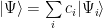
Since I limited the discussion to the simple 1D chain, imagine a chain formed by sites with spin. A state of such chain is in the space obtained as a tensor product of local spaces (for each individual spin). The state can be decomposed as:

$\lvert\Psi\rangle=\sum\limits_{i_1,...,i_n} C^{i_1,...,i_n}\lvert i_1,...,i_n\rangle$

where each index runs over the local basis ( $i_1$ over the basis of site 1 and so on). C is a nasty object (let’s call it a tensor from now on) which has $d^n$ elements. The exponential increase of the state space makes this very hard to deal with.
The idea would be to somehow find a simplification. The easiest one is to consider:

$C^{i_1,...,i_n}=C^{i_1}C^{i_2}...C^{i_n}$

That is, a simple product state. This is the approximation used in mean field theory, the sites do not interact (directly) with the other sites, only with the mean field. The complexity drops from $d^n$ to $dn$ or even d if there is translational symmetry.
Quite nice, but this approximation does not work in general. So let’s find something better.

The idea is to separate out the chain in two and apply Singular Value Decomposition on it. Please visit the DMRG post for details, for DMRG, SVD is also very important.
I’ll start with the leftmost site in the chain, you could start with the rightmost site, or you could split the chain in two – you can call one part ‘system’, one ‘environment’, to see the link with DMRG. Keeping the singular values separately will lead you to the Vidal decomposition, I’ll simply multiply S into $V^\dagger$ to keep things simple. So, by grouping all indices but the first one into a single index we get a matrix with elements $C^{i_1,(i_2...i_n)}$ on which one can apply singular value decomposition:

$C = USV^\dagger$

The S matrix can be multiplied with the $V^\dagger$ one and the decomposition for a tensor element becomes:

$C^{i_1,(i_2...i_n)}=\sum\limits_{v_1}U^{i_1}_{v_1}\tilde{C}^{v_1,(i_2...i_n)}$

Let’s add a dummy index for U, too, its role will be obvious soon:

$C^{i_1,(i_2...i_n)}=\sum\limits_{v_1}U^{i_1}_{1, v_1}\tilde{C}^{v_1,(i_2...i_n)}$

Now let’s perform SVD again for $\tilde{C}$ , grouping first two indices together into one and the remaining ones into the other to make a matrix (the procedure is called reshaping, by the way):

$\tilde{C}^{(v_1,i_2),(i_3...i_n)}=\sum\limits_{v_2}U^{v_1, i_2}_{v_2}\tilde{\tilde{C}}^{v_2,(i_3...i_n)}$

By arranging indices, inserting in the previous one and removing one tilde sign (so $\tilde{\tilde{C}}$ is now renamed $\tilde{C}$ ):

$C^{i_1...i_n}=\sum\limits_{v_1, v_2}U^{i_1}_{1, v_1} U^{i_2}_{v_1, v_2}\tilde{C}^{v_2,(i_3...i_n)}$

By repeating the procedure one finally gets:

$C^{i_1...i_n}=\sum\limits_{v_1 ... v_n}U^{i_1}_{1, v_1} U^{i_2}_{v_1, v_2} U^{i_3}_{v_2, v_3} ... U^{i_n}_{v_n, 1}$

What we have now is just a product of matrices. By considering the dimensionality, which I did not discuss and I advise you to look into the references for details, it’s not immediately obvious how this could help.
But we performed SVD as in DMRG and with the help of the area law we can truncate those matrices. Please check out the links for details and maybe also the DMRG post.
This way the computations will simplify tremendously.

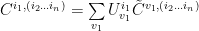
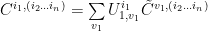
The matrix decomposition is not unique, one can insert 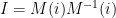$I=M(i)M^{-1}(i)$ to change the decomposition, but some decompositions are more useful than others, so the left and right and mixed canonical are used.

To summarize, we ended up with a set of d matrices for each site, d being the dimensionality of the local space, that is, for a 1/2 spin site d=2 and we have two matrices, one for spin up and one for spin down for each site.
The indices I noted with ‘v’ are called virtual indices (or valence indexes), the ones noted with ‘i’, physical indices, they select the matrix, in our 1/2 spin case, the spin down or spin up matrix.

This is only a brief presentation of the product matrix decomposition, if one is not familiar with it already, he should check also the valence bond picture and the usage in context of DMRG.
There is also a very useful graphical representation which is used a lot, one should also check it out. In that representation, for a site (which is not at an end), there is a circle with three legs sticking out: two horizontal ones corresponding to virtual indices and a vertical one corresponding to the physical one. Connected legs means summing over.

Simple examples

To get a feeling of how the MPS looks like, I thought it might be useful to mention some trivial cases. First, for a case when there is a simple product state, let’s say all spins up: in this case the matrices have the dimension 1×1 and all matrices for spin down are 0, all for spin up are one, so the two matrices for a site are 0 and 1. For a case where the state cannot be written as a simple product state, let’s consider the superposition between all spins up and all spins down:

$\lvert\Psi\rangle=\lvert\uparrow\uparrow ... \uparrow\rangle+\lvert\downarrow\downarrow ... \downarrow\rangle$

In this case for each site there is a matrix for spin up, one for spin down, which have the form:

$\left(\begin{array}{cc} 1 & 0\\ 0 & 0 \end{array}\right)$

and

$\left(\begin{array}{cc} 0 & 0\\ 0 & 1 \end{array}\right)$

Matrix Product Operators

An operator is more complex than a state:

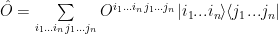
$\hat{O} = \sum\limits_{i_1...i_n j_1 ... j_n} O^{i_1...i_n j_1 ... j_n} |i_1...i_n\rangle\langle j_1...j_n|$

We have an uglier tensor but indices can be arranged by grouping them together:

$\hat{O} = \sum\limits_{i_1 j_1...i_n j_n} O^{(i_1 j_1)...(i_n j_n)} |i_1...i_n\rangle\langle j_1...j_n|$

By considering each pair (ij) as a single index one can follow the same procedure as before to decompose it into a matrix product. The difference is that one ends up with two physical indices instead of one, so the graphical representation has two vertical and two horizontal legs/site. For the simplest case when the operator acts on a single site, for all the other sites the operator matrices are trivial.
It’s beyond the scope of this post to present in detail everything, for the details please check at least DMRG: Ground States, Time Evolution, and Spectral Functions⁸.

Suzuki-Trotter expansion

Let’s assume the Hamiltonian having only nearest neighbor interaction and on site terms, in the form:

$H = \sum\limits_{i}(T_{1,i}+T_{2,(i,i+1)})$

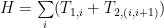
The time evolution operator is:

$U = e^{-i H t}$

The time can be divided into n infinitesimal periods, to have:

$U = (e^{-i H t/n})^n$

The Hamiltonian can be written as a sum of even and odd terms:

$H = H_{odd} + H_{even} = \sum\limits_{i even}(T_{1,i}+T_{2,(i,i+1)}) + \sum\limits_{i odd}(T_{1,i}+T_{2,(i,i+1)}) = \sum\limits_{i even}E_i + \sum\limits_{i odd}O_i$

The reason is that the even terms commute among themselves, also the odd terms commute among themselves, although an even term and an odd term do not necessarily commute. So separately for the even and odd parts:

$e^{-i H_{even} t/n} = \prod\limits_{ieven} e^{-iE_i t/n}$

And similarly for the odd part of the Hamiltonian.

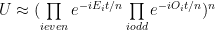
The first order approximation is:

$e^{-i H t/n} = e^{-i(H_{odd} + H_{even})t/n}\approx e^{-iH_{odd}t/n}e^{-i H_{even}t/n}$

The approximation is exact when n goes to infinity. It’s only an approximation because terms from the even part do not commute with terms from the odd part, by the way.

Time Evolution

We have above all ingredients to perform a time evolution. Putting it all together we have:

$U \approx (\prod\limits_{ieven} e^{-iE_i t/n} \prod\limits_{iodd} e^{-iO_i t/n})^n$

This can be translated into words approximately as: Apply all even evolution operator terms on the state then all the odd terms. Repeat the procedure n times to evolve the state to time t.

Imaginary Time

One can perform an imaginary time evolution by absorbing i into time, transforming it into imaginary time (see: Wick rotation). The evolution operator becomes:

$U = e^{-iHt} = e^{-H\tau}$

The assumption is that we have a ground state separated by an energy gap.
Let’s start with a random state, the only requirement being to have a non-zero component along the ground state vector. We can write the state using the Hamiltonian eigenstates:

$|\Psi\rangle=\sum\limits_i c_i|\Psi_i\rangle$

with $|\Psi_0\rangle$ being the ground state vector. The states have the corresponding eigenvalues $E_i$ , $E_0$ being the ground state energy. By applying the imaginary time evolution operator on the initial state for a sufficiently long time:

$U|\Psi\rangle=\sum\limits_i c_i e^{-E_i \tau}|\Psi_i\rangle$

the ground state is amplified (the coefficient gets bigger and bigger) while all the others are getting smaller in comparison.

The blowup of the ground state coefficient is compensated by normalizing the evolved state:

$|\Psi_0\rangle\approx\frac{U |\Psi\rangle}{|U |\Psi\rangle|^2}$

The approximation becomes exact in the limit of $\tau$ going to infinity.

Here is another imaginary time evolution presentation for the Schrödinger equation in a simpler context: Numerical solution of PDE:s, Part 5: Schrödinger equation in imaginary time¹⁶

The Infinite Chain

For the details I’ll let you look in the Vidal iTEBD paper, I’ll present only the main idea:

The infinite chain has translation symmetry, so instead of taking into account all sites one can get away by considering only the sites i and i+1, the chain looks everywhere the same, anyway. First the even evolution term is applied to those, then the i site is moved to the i+2 position and the odd evolution term is applied on sites i+1 and i+2 (equivalently, the sites are swapped and the odd term is applied on sites i and i+1). Then the process is repeated. This will become much clear in the code presentation below, also if you take a look in the iTEBD paper⁵.

The Code

Generalities

The program is a quite standard mfc application, very similar with other applications I presented on this blog, so I won’t bother to describe it in detail. You have the standard doc/view and the application object. I got from the other projects the number edit control and the chart class, as usual there is an options object in the application that allows saving/loading into/from registry, there is the options property sheet and pages and a computation thread which lets the application be responsive while doing the calculations.
Everything important for the topic is in the TEBD namespace.

Operators

The operators are implemented in the TEBD::Operators namespace. I simply copied them from the DMRG project (so you’ll see some remains from there – also from the NRG project – despite not being used in the current project) and changed and extended them to fit to this project. The operator classes are just wrappers around Eigen¹⁷ matrices with some functionality added. The matrices are initialized to the proper value in constructors.
The currently used Hamiltonian is:

class Heisenberg : public Hamiltonian<double>
{
public:
    Heisenberg(double Jx, double Jy, double Jz, double Bx = 0, double Bz = 0);
};

class Heisenberg : public Hamiltonian<double>

{

public:

Heisenberg(double Jx, double Jy, double Jz, double Bx = 0, double Bz = 0);

};

with its constructor implementation being:

inline Heisenberg::Heisenberg(double Jx, double Jy, double Jz, double Bx, double Bz)
    : Hamiltonian<double>(2)
{
    Operators::SxOneHalf<double> sx;
    Operators::SyOneHalf<double> sy;
    Operators::SzOneHalf<double> sz;
            
    matrix = - (Jx * Operators::Operator<double>::KroneckerProduct(sx.matrix, sx.matrix)
        - Jy * Operators::Operator<double>::KroneckerProduct(sy.matrix, sy.matrix)
        + Jz * Operators::Operator<double>::KroneckerProduct(sz.matrix, sz.matrix)
        + Bx/2 * (Operators::Operator<double>::IdentityKronecker(2, sx.matrix) + Operators::Operator<double>::KroneckerProductWithIdentity(sx.matrix, 2))
        + Bz/2 * (Operators::Operator<double>::IdentityKronecker(2, sz.matrix) + Operators::Operator<double>::KroneckerProductWithIdentity(sz.matrix, 2)));
}

inline Heisenberg::Heisenberg(double Jx, double Jy, double Jz, double Bx, double Bz)

: Hamiltonian<double>(2)

{

Operators::SxOneHalf<double> sx;

Operators::SyOneHalf<double> sy;

Operators::SzOneHalf<double> sz;

matrix = - (Jx * Operators::Operator<double>::KroneckerProduct(sx.matrix, sx.matrix)

- Jy * Operators::Operator<double>::KroneckerProduct(sy.matrix, sy.matrix)

+ Jz * Operators::Operator<double>::KroneckerProduct(sz.matrix, sz.matrix)

+ Bx/2 * (Operators::Operator<double>::IdentityKronecker(2, sx.matrix) + Operators::Operator<double>::KroneckerProductWithIdentity(sx.matrix, 2))

+ Bz/2 * (Operators::Operator<double>::IdentityKronecker(2, sz.matrix) + Operators::Operator<double>::KroneckerProductWithIdentity(sz.matrix, 2)));

}

I guess the code should be explicit enough. It’s just the Hamiltonian for the two sites from iTEBD. This could also be used for the finite length chain, the algorithm is very similar, just instead of two sites which are ‘swapped’ each step, the finite algorithm walks over all sites (first over all those having ‘odd’ interactions, then over those having ‘even’ interactions).

The rest of the operators code was already described in other posts of this blog and is straightforward. Something which is new and is worth mentioning is the exponentiation of an operator, implemented in the DiagonalizableOperator class:

inline Eigen::MatrixXcd ComplexExponentiate(double tau)
{
    Diagonalize();

    const Operator<T>::OperatorMatrix& eigenV = eigenvectors();
    const Operator<T>::OperatorVector& eigenv = eigenvalues();

    Eigen::VectorXcd result = Eigen::VectorXcd(eigenv.size());

    for (int i = 0; i < eigenv.size(); ++i)
        result(i) = std::exp(std::complex<double>(0, -1) * tau * eigenv(i));

    return eigenV * result.asDiagonal() * eigenV.transpose();
}

inline Eigen::MatrixXcd ComplexExponentiate(double tau)

{

Diagonalize();

const Operator<T>::OperatorMatrix& eigenV = eigenvectors();

const Operator<T>::OperatorVector& eigenv = eigenvalues();

Eigen::VectorXcd result = Eigen::VectorXcd(eigenv.size());

for (int i = 0; i < eigenv.size(); ++i)

result(i) = std::exp(std::complex<double>(0, -1) * tau * eigenv(i));

return eigenV * result.asDiagonal() * eigenV.transpose();

}

There is another similar method which is used for the imaginary time variant.
The code is used to calculate $e^{-iHt}$ , H being the Hamiltonian operator matrix.
The idea is to diagonalize the matrix, calculate the exponentials of the eigenvalues then bring the matrix back to the original basis using the eigenvectors. More details on Wikipedia page.

iTEBD code

The matrix product state is stored in the an iMPS object, declared as:

template<typename T, unsigned int D = 2> class iMPS
{
public:
    iMPS(unsigned int chi = 10);
    virtual ~iMPS();

    virtual void InitRandomState();
    void InitNeel();

    Eigen::Tensor<T, 3> Gamma1;
    Eigen::Tensor<T, 3> Gamma2;

    typename Operators::Operator<double>::OperatorVector lambda1;
    typename Operators::Operator<double>::OperatorVector lambda2;
};

template<typename T, unsigned int D = 2> class iMPS

{

public:

iMPS(unsigned int chi = 10);

virtual ~iMPS();

virtual void InitRandomState();

void InitNeel();

Eigen::Tensor<T, 3> Gamma1;

Eigen::Tensor<T, 3> Gamma2;

typename Operators::Operator<double>::OperatorVector lambda1;

typename Operators::Operator<double>::OperatorVector lambda2;

};

It’s not very complicated: it just stores the gamma tensors and lambda values for two sites and has methods to initialize the state to a random one or to a Neel state (translation symmetrized by averaging).

As a side note, having it implemented for the finite chain should not be hard at all: instead of only two sites, have values for all sites, in vectors. Maybe the lambda values could be multiplied into the site matrices, but I didn’t give that much thought.

By the way, the code uses the ‘unsupported’ tensor library included in Eigen. Despite being unsupported, I guess it’s good enough since it’s used in TensorFlow. I had some troubles with reshaping and I ended up implementing that myself (along with shuffling).

Most of the computation code is in the iTEBD implementation. Evolution, both in real and imaginary time, is implemented this way:

template<typename T, unsigned int D> 
double iTEBD<T, D>::CalculateImaginaryTimeEvolution(Operators::Hamiltonian<double>& H, unsigned int steps, double delta)
{
    m_iMPS.InitRandomState();

    Operators::Operator<T>::OperatorMatrix Umatrix = GetImaginaryTimeEvolutionOperatorMatrix(H, delta);
    Eigen::Tensor<T, 4> U = GetEvolutionTensor(Umatrix);
        
    isRealTimeEvolution = false;
    Calculate(U, steps);

    return GetEnergy(delta, thetaMatrix);
}

template<typename T, unsigned int D> 
void iTEBD<T, D>::CalculateRealTimeEvolution(Operators::Hamiltonian<double>& H, unsigned int steps, double delta)
{
    Eigen::MatrixXcd Umatrix = GetRealTimeEvolutionOperatorMatrix(H, delta);
    Eigen::Tensor<T, 4> U = GetEvolutionTensor(Umatrix);

    isRealTimeEvolution = true;
    Calculate(U, steps);
}

template<typename T, unsigned int D>

double iTEBD<T, D>::CalculateImaginaryTimeEvolution(Operators::Hamiltonian<double>& H, unsigned int steps, double delta)

{

m_iMPS.InitRandomState();

Operators::Operator<T>::OperatorMatrix Umatrix = GetImaginaryTimeEvolutionOperatorMatrix(H, delta);

Eigen::Tensor<T, 4> U = GetEvolutionTensor(Umatrix);

isRealTimeEvolution = false;

Calculate(U, steps);

return GetEnergy(delta, thetaMatrix);

}

template<typename T, unsigned int D>

void iTEBD<T, D>::CalculateRealTimeEvolution(Operators::Hamiltonian<double>& H, unsigned int steps, double delta)

{

Eigen::MatrixXcd Umatrix = GetRealTimeEvolutionOperatorMatrix(H, delta);

Eigen::Tensor<T, 4> U = GetEvolutionTensor(Umatrix);

isRealTimeEvolution = true;

Calculate(U, steps);

}

There is not much difference between evolution in imaginary time and real time: the difference is in the evolution operator and a flag that indicates what kind of evolution is, and that’s about it.

inline static typename Operators::Operator<double>::OperatorMatrix GetImaginaryTimeEvolutionOperatorMatrix(Operators::Hamiltonian<double>& H, double deltat)
{
    return H.Exponentiate(deltat);
}

inline static Eigen::MatrixXcd GetRealTimeEvolutionOperatorMatrix(Operators::Hamiltonian<double>& H, double deltat)
{
    return H.ComplexExponentiate(deltat);
}

inline static typename Operators::Operator<double>::OperatorMatrix GetImaginaryTimeEvolutionOperatorMatrix(Operators::Hamiltonian<double>& H, double deltat)

{

return H.Exponentiate(deltat);

}

inline static Eigen::MatrixXcd GetRealTimeEvolutionOperatorMatrix(Operators::Hamiltonian<double>& H, double deltat)

{

return H.ComplexExponentiate(deltat);

}

As expected, the imaginary and real time evolution operators are nothing more than already described above.
GetEvolutionTensor just converts the operator matrix into a tensor ready to be applied, I’ll let you look into the code for its implementation. It’s one place where reshaping and reshuffling are implemented by me instead of using the tensor library.

Now let’s see the main part:

template<typename T, unsigned int D> 
void iTEBD<T, D>::Calculate(const Eigen::Tensor<T, 4> &U, unsigned int steps)
{
    for (unsigned int step = 0; step < steps; ++step)
    {
        bool odd = (1 == step % 2);

        Eigen::Tensor<T, 2> lambdaA(m_chi, m_chi);
        Eigen::Tensor<T, 2> lambdaB(m_chi, m_chi);

        lambdaA.setZero();
        lambdaB.setZero();

        Eigen::Tensor<T, 3> &gammaA = odd ? m_iMPS.Gamma2 : m_iMPS.Gamma1;
        Eigen::Tensor<T, 3> &gammaB = odd ? m_iMPS.Gamma1 : m_iMPS.Gamma2;

        for (unsigned int i = 0; i < m_chi; ++i)
        {
            lambdaA(i, i) = odd ? m_iMPS.lambda2(i) : m_iMPS.lambda1(i);
            lambdaB(i, i) = odd ? m_iMPS.lambda1(i) : m_iMPS.lambda2(i);
        }

        // construct theta

        // this does the tensor network contraction as in fig 3, (i)->(ii) from iTEBD Vidal paper
        Eigen::Tensor<T, 4> thetabar = ConstructTheta(lambdaA, lambdaB, gammaA, gammaB, U);

        // ***********************************************************************************************************


        // get it into a matrix for SVD - use JacobiSVD

        // the theta tensor is now decomposed using SVD (as in (ii)->(iii) in fig 3 in Vidal iTEBD paper) and then 
        // the tensor network is rebuilt as in (iii)->(iv)->(v) from fig 3 Vidal 2008

        thetaMatrix = ReshapeTheta(thetabar);

        Eigen::JacobiSVD<Operators::Operator<T>::OperatorMatrix> SVD(thetaMatrix, Eigen::DecompositionOptions::ComputeFullU | Eigen::DecompositionOptions::ComputeFullV);

        Operators::Operator<T>::OperatorMatrix Umatrix = SVD.matrixU().block(0, 0, D * m_chi, m_chi);
        Operators::Operator<T>::OperatorMatrix Vmatrix = SVD.matrixV().block(0, 0, D * m_chi, m_chi).adjoint();
            
        Operators::Operator<double>::OperatorVector Svalues = SVD.singularValues();

        for (unsigned int i = 0; i < m_chi; ++i)
        {
            double val = Svalues(i);

            if (odd) m_iMPS.lambda2(i) = val;
            else m_iMPS.lambda1(i) = val;

            if (abs(lambdaB(i,i)) > 1E-10) 
                lambdaB(i, i) = 1. / lambdaB(i, i);     
            else lambdaB(i, i) = 0;
        }

        if (odd) m_iMPS.lambda2.normalize();
        else m_iMPS.lambda1.normalize();

        SetNewGammas(m_chi, lambdaB, Umatrix, Vmatrix, gammaA, gammaB); 

        // now compute 'measurements'
        // this program uses a 'trick' by reusing the already contracted tensor network
            
        if (odd && isRealTimeEvolution && m_TwoSitesOperators.size() > 0)
            ComputeOperators(thetabar);
    }
}

template<typename T, unsigned int D>

void iTEBD<T, D>::Calculate(const Eigen::Tensor<T, 4> &U, unsigned int steps)

{

for (unsigned int step = 0; step < steps; ++step)

{

bool odd = (1 == step % 2);

Eigen::Tensor<T, 2> lambdaA(m_chi, m_chi);

Eigen::Tensor<T, 2> lambdaB(m_chi, m_chi);

lambdaA.setZero();

lambdaB.setZero();

Eigen::Tensor<T, 3> &gammaA = odd ? m_iMPS.Gamma2 : m_iMPS.Gamma1;

Eigen::Tensor<T, 3> &gammaB = odd ? m_iMPS.Gamma1 : m_iMPS.Gamma2;

for (unsigned int i = 0; i < m_chi; ++i)

{

lambdaA(i, i) = odd ? m_iMPS.lambda2(i) : m_iMPS.lambda1(i);

lambdaB(i, i) = odd ? m_iMPS.lambda1(i) : m_iMPS.lambda2(i);

}

// construct theta

// this does the tensor network contraction as in fig 3, (i)->(ii) from iTEBD Vidal paper

Eigen::Tensor<T, 4> thetabar = ConstructTheta(lambdaA, lambdaB, gammaA, gammaB, U);

// ***********************************************************************************************************

// get it into a matrix for SVD - use JacobiSVD

// the theta tensor is now decomposed using SVD (as in (ii)->(iii) in fig 3 in Vidal iTEBD paper) and then

// the tensor network is rebuilt as in (iii)->(iv)->(v) from fig 3 Vidal 2008

thetaMatrix = ReshapeTheta(thetabar);

Eigen::JacobiSVD<Operators::Operator<T>::OperatorMatrix> SVD(thetaMatrix, Eigen::DecompositionOptions::ComputeFullU | Eigen::DecompositionOptions::ComputeFullV);

Operators::Operator<T>::OperatorMatrix Umatrix = SVD.matrixU().block(0, 0, D * m_chi, m_chi);

Operators::Operator<T>::OperatorMatrix Vmatrix = SVD.matrixV().block(0, 0, D * m_chi, m_chi).adjoint();

Operators::Operator<double>::OperatorVector Svalues = SVD.singularValues();

for (unsigned int i = 0; i < m_chi; ++i)

{

double val = Svalues(i);

if (odd) m_iMPS.lambda2(i) = val;

else m_iMPS.lambda1(i) = val;

if (abs(lambdaB(i,i)) > 1E-10)

lambdaB(i, i) = 1. / lambdaB(i, i);

else lambdaB(i, i) = 0;

}

if (odd) m_iMPS.lambda2.normalize();

else m_iMPS.lambda1.normalize();

SetNewGammas(m_chi, lambdaB, Umatrix, Vmatrix, gammaA, gammaB);

// now compute 'measurements'

// this program uses a 'trick' by reusing the already contracted tensor network

if (odd && isRealTimeEvolution && m_TwoSitesOperators.size() > 0)

ComputeOperators(thetabar);

}

It looks more complicated than it should, but it’s not very bid deal:

There is a for loop which performs a number of steps of evolution (one could do better by changing the step size and matrices size along evolution to be able to have more accuracy along a longer time evolution, but I’ll refer you to documentation for such subtleties). In the for loop, five things are happening:
* first, the site are swapped if it’s an ‘odd’ step. The first portion of the code down to the // construct theta comment does that, along with getting the lambda values into tensors to deal with them easier in further computations.
* second, the lambda and gamma tensors are contracted together to obtain a ‘four legs’ tensor and then the evolution tensor is applied (contracted with the result). All those happen in the ConstructTheta call
* third, a singular value decomposition is performed after the four legs tensor is reshaped into a matrix
* fourth, the result of SVD is split back into the sites matrices and lambda values. As a detail, the site tensor has three legs, the second one being the physical one (that is, that index selects the matrix). This is implemented after the call to singularValues down to (and including) the call to SetNewGammas
* last, if there are ‘measurement’ operators to compute, compute them

Here is the ConstructTheta implementation:

// this does the tensor network contraction as in fig 3, (i)->(ii) from iTEBD Vidal paper
template<typename T, unsigned int D> 
Eigen::Tensor<T, 4> iTEBD<T, D>::ConstructTheta(const Eigen::Tensor<T, 2>& lambdaA, const Eigen::Tensor<T, 2>& lambdaB, const Eigen::Tensor<T, 3>& gammaA, const Eigen::Tensor<T, 3>& gammaB, const Eigen::Tensor<T, 4>& U)
{
    Eigen::Tensor<T, 4> theta = ContractTwoSites(lambdaA, lambdaB, gammaA, gammaB);

    // apply time evolution operator
    typedef Eigen::Tensor<T, 4>::DimensionPair DimPair;

    // from theta the physical indexes are contracted out
    // the last two become the physical indexes

    const Eigen::array<DimPair, 2> product_dim{ DimPair(1, 0), DimPair(2, 1) };               
        
    // this applies the time evolution operator U
    return theta.contract(U, product_dim);
}

// this does the tensor network contraction as in fig 3, (i)->(ii) from iTEBD Vidal paper

template<typename T, unsigned int D>

Eigen::Tensor<T, 4> iTEBD<T, D>::ConstructTheta(const Eigen::Tensor<T, 2>& lambdaA, const Eigen::Tensor<T, 2>& lambdaB, const Eigen::Tensor<T, 3>& gammaA, const Eigen::Tensor<T, 3>& gammaB, const Eigen::Tensor<T, 4>& U)

{

Eigen::Tensor<T, 4> theta = ContractTwoSites(lambdaA, lambdaB, gammaA, gammaB);

// apply time evolution operator

typedef Eigen::Tensor<T, 4>::DimensionPair DimPair;

// from theta the physical indexes are contracted out

// the last two become the physical indexes

const Eigen::array<DimPair, 2> product_dim{ DimPair(1, 0), DimPair(2, 1) };

// this applies the time evolution operator U

return theta.contract(U, product_dim);

}

The last line applies the evolution operator, the rest is delegated to ContractTwoSites:

template<typename T, unsigned int D> 
Eigen::Tensor<T, 4> iTEBD<T, D>::ContractTwoSites(const Eigen::Tensor<T, 2>& lambdaA, const Eigen::Tensor<T, 2>& lambdaB, const Eigen::Tensor<T, 3>& gammaA, const Eigen::Tensor<T, 3>& gammaB)
{
    // construct theta

    // contract lambda on the left with the first gamma
    // the resulting tensor has three legs, 1 is the physical one
    const Eigen::array<Eigen::IndexPair<int>, 1> product_dims1{ Eigen::IndexPair<int>(1, 0) };
    Eigen::Tensor<T, 3> thetaint = lambdaB.contract(gammaA, product_dims1);

    // contract the result with the lambda in the middle
    // the resulting tensor has three legs, 1 is the physical one
    const Eigen::array<Eigen::IndexPair<int>, 1> product_dims2{ Eigen::IndexPair<int>(2, 0) };
    thetaint = thetaint.contract(lambdaA, product_dims2).eval();

    // contract the result with the next gamma
    // the resulting tensor has four legs, 1 and 2 are the physical ones
    const Eigen::array<Eigen::IndexPair<int>, 1> product_dims3{ Eigen::IndexPair<int>(2, 0) };
    Eigen::Tensor<T, 4> theta = thetaint.contract(gammaB, product_dims3);

    // contract the result with the lambda on the right
    // the resulting tensor has four legs, 1 and 2 are the physical ones
    const Eigen::array<Eigen::IndexPair<int>, 1> product_dims4{ Eigen::IndexPair<int>(3, 0) };
        
    return theta.contract(lambdaB, product_dims4);      
}

template<typename T, unsigned int D>

Eigen::Tensor<T, 4> iTEBD<T, D>::ContractTwoSites(const Eigen::Tensor<T, 2>& lambdaA, const Eigen::Tensor<T, 2>& lambdaB, const Eigen::Tensor<T, 3>& gammaA, const Eigen::Tensor<T, 3>& gammaB)

{

// construct theta

// contract lambda on the left with the first gamma

// the resulting tensor has three legs, 1 is the physical one

const Eigen::array<Eigen::IndexPair<int>, 1> product_dims1{ Eigen::IndexPair<int>(1, 0) };

Eigen::Tensor<T, 3> thetaint = lambdaB.contract(gammaA, product_dims1);

// contract the result with the lambda in the middle

// the resulting tensor has three legs, 1 is the physical one

const Eigen::array<Eigen::IndexPair<int>, 1> product_dims2{ Eigen::IndexPair<int>(2, 0) };

thetaint = thetaint.contract(lambdaA, product_dims2).eval();

// contract the result with the next gamma

// the resulting tensor has four legs, 1 and 2 are the physical ones

const Eigen::array<Eigen::IndexPair<int>, 1> product_dims3{ Eigen::IndexPair<int>(2, 0) };

Eigen::Tensor<T, 4> theta = thetaint.contract(gammaB, product_dims3);

// contract the result with the lambda on the right

// the resulting tensor has four legs, 1 and 2 are the physical ones

const Eigen::array<Eigen::IndexPair<int>, 1> product_dims4{ Eigen::IndexPair<int>(3, 0) };

return theta.contract(lambdaB, product_dims4);

}

There isn’t much more to say here, the comments should be clear enough.

I’ll let you look over the project source¹ for the code that is not presented here, it shouldn’t be hard to figure out by now.

A result

I tested the code with some results I found for both imaginary time evolution and real time evolution, I’ll present here only one result I reproduced with the program:

It’s the magnetization real time evolution from Classical simulation of infinite-size quantum lattice systems in one spatial dimension⁵, fig 6, for an infinite Ising chain with transverse magnetic field with initial state obtained by imaginary time evolution.

Conclusion

That’s about it for now. I guess the program should be easily changed to work with spin-1 Hamiltonians and with some more effort the finite chain could be implemented. I might implement both in the future, but for this post this is enough.
If you find any issues or have suggestions, please let me know.

CodeProject

TEBD program in the GitHub repository. ↩ ↩
A class of ansatz wave functions for 1D spin systems and their relation to DMRG by Stefan Rommer and Stellan Ostlund. ↩
Efficient classical simulation of slightly entangled quantum computations The first article on TEBD by Vidal. ↩
Efficient simulation of one-dimensional quantum many-body systems The second one on TEBD by Vidal. ↩
Classical simulation of infinite-size quantum lattice systems in one spatial dimension iTEBD by Vidal. ↩ ↩ ↩
Matrix Product States, Projected Entangled Pair States, and variational renormalization group methods for quantum spin systems Review by F. Verstraete, J.I. Cirac and V. Murg ↩
The density-matrix renormalization group in the age of matrix product states Review by Ulrich Schollwock ↩
DMRG: Ground States, Time Evolution, and Spectral Functions by Ulrich Schollwock ↩ ↩
A Practical Introduction to Tensor Networks: Matrix Product States and Projected Entangled Pair States by Roman Orus ↩
Matrix Product State Representations by D. Perez-Garcia, F. Verstraete, M.M. Wolf, J.I. Cirac ↩
Efficient Numerical Simulations Using Matrix-Product States by Frank Pollmann ↩
Finite automata for caching in matrix product algorithms by Gregory M. Crosswhite and Dave Bacon ↩
Numerical Time Evolution of 1D Quantum Systems by Elias Rabel ↩
Tensor network states for the description of quantum many-body systems by Thorsten Bernd Wahl ↩
ITensor Intelligent Tensor library ↩
Numerical solution of PDE:s, Part 5: Schrödinger equation in imaginary time A blog entry I found on the net. ↩
Eigen The matrix library. ↩

Introduction

Links

On this blog

The most important for the topic

Reviews, Lectures and so on

Software

A Video Lecture

Simplifications

Matrix Product States

Simple examples

Matrix Product Operators

Suzuki-Trotter expansion

Time Evolution

Imaginary Time

The Infinite Chain

The Code

Generalities

Operators

iTEBD code

A result

Conclusion

Like this:

Related

Leave a Reply (for privacy concerns, please read the Privacy Policy Page accessible from the top menu)Cancel reply

Introduction

Links

On this blog

The most important for the topic

Reviews, Lectures and so on

Software

A Video Lecture

Simplifications

Matrix Product States

Simple examples

Matrix Product Operators

Suzuki-Trotter expansion

Time Evolution

Imaginary Time

The Infinite Chain

The Code

Generalities

Operators

iTEBD code

A result

Conclusion

Share this:

Like this:

Related

Leave a Reply (for privacy concerns, please read the Privacy Policy Page accessible from the top menu)Cancel reply