
Introduction
When I started this blog I already expected to have projects that use the Fast Fourier Transform. I actually wrote down several topic ideas for the blog, both solving the Poisson equation and the subject this post will lead to were there, too. I already mentioned in the Relaxation Method post that one can use the Discrete Fourier Transform to solve the problem faster and here it is, as an intermediate step leading to at least one project on Density Functional Theory.
I won’t discuss here the Fast Fourier Transform, I already have the previous post for that, so the classes that deal with FFT will not be presented here. I just copied them from the last project and used them. I will reuse them in the DFT project(s) as well, along with the Poisson solver (probably with changes).
This post also introduces VTK, The Visualization Toolkit1, a library which I will also use in future projects. Even for this project, where I could implement those surfaces easily with OpenGL – but not so easily the axes behaving like those from VTK, an implementation which could take quite long and be quite boring – the library saved quite a bit of time. VTK allows very impressive visualizations of scientific data saving a lot of time (I’m told that the library has way more than 1000 years of developer time in it, obviously I cannot beat it in reasonable amount of time). Using it will allow me to focus on the parts related with the blog topic more and will allow me make some projects that I would avoid otherwise due of the visualization complexities, as I avoided for example the 3D flow for the Lattice Boltzmann post. I know it’s nicer to just download the code and be able to compile it, with as little dependencies as possible, but having the VTK dependency brings up too many advantages to avoid it. I might use just OpenGL in the future for certain projects, but for complex 3D visualizations or even charting, except very simple charts as I already used in projects for this blog, I’ll use VTK.
For this post I implemented a Poisson equation solver using a spectral method. Here is the program in action:
What you see in there is just a section halfway through the 3D volume, with periodic boundary conditions. In the left view I represented the charge density, generated with two gaussians, in the right view is the solution to the Poisson equation. The source code for the project is on GitHub2.
Links
I didn’t want to reveal the purpose of bringing up the FFT themes on the blog yet, because I thought that I might just give up implementing the DFT project for various reasons, but I thought it would be nice to give some links I looked into while having a DFT prototype implemented. Incidentally the featured image at the top of the post is an Octave chart I generated while implementing the DFT prototype.
At first I wanted to simply write an easy DFT project using a real space discretization. I already implemented a simple DFT program – proof of concept style – that way, some time ago. Discretization of the real space and using a simple method like the finite difference method is not a bad way to start, the method is simple to understand and implement. But if you want some performance it might not be the best way, so this time I thought to use Gaussian orbitals similarly as for the Hartree-Fock project. Then I thought I might want to implement sometime a project for a crystal, in which case the periodic boundary conditions come into play. In such a case, due of periodicity, the plane wave basis is very good and besides, it brings something new for this blog. With the help of the Hartree-Fock posts and the DFT ones, there should be enough information to be able to implement a DFT program using Gaussian orbitals, too.
So, I decided to go the plane waves basis way, then I started looking for some info on the net about it. I knew the theory, knew some things about implementation but I wanted to look into the details a little more, the devil is in the details. I started working on the Hartree-Fock project before having all the details clear and it took me more time than I anticipated. Of course there are plenty of lectures on DFT, I’ll point to those in the posts about DFT, but they touch only the theory. With a little search on YouTube I found something more appropriate, from Cornell University:
The first two lectures and a part of the third are relevant to this project, if I recall correctly.
Unfortunately it misses some parts, but with the help from the links the gaps can be filled. Here is a very useful link (there is a link mentioned in the lecture, that’s how I reached this link): Arias Classes3. You want to look into the Phys 7654 Practical DFT folders, preferably the latest. You’ll find there readings and very importantly, assignments. One of the theory papers is also found on arxiv: New Algebraic Formulation of Density Functional Calculation4. I just implemented the assignments in Octave to be sure it’s something relatively easy to do, now I only have to ‘translate’ them to C++ and of course, have a nicer visualization if possible. The project for this blog post corresponds to the first assignment, but computations are simplified to make the project easier to understand. There is no ‘overlap’ operator in the C++ project (the basis is orthogonal) and also I got rid of various cI, cIdag, cJ, cJdag, forward and inverse FFT is sufficient for this project.
Some theory
Poisson equation appears in various contexts, but for now we are interested in the electromagnetic field. The equation is:

Where 
For more details, please check this page: Mathematical description of the electromagnetic field.
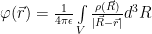
Not surprisingly, because of linearity, the field is given by the ‘sum’ (the integral) of the fields generated by each ‘point’ charge in the volume. You could try to solve the integral numerically and for a few point charges it wouldn’t be so difficult. Also for a limited number of localized charge distributions, with spherical symmetry, you could use some tricks to simplify things, but in general, this integral is quite hard to solve in real space. For 3D if you cut the volume in 


You can interchange the Laplace operator with the integral and more, since the operator does not act on k, skip over 


The code
The FFT code is in the Fourier namespace and I already mentioned it in the previous post. I also used in this project the Vector3D<T> class I used in other projects. I think it should be pretty clear what it does, I won’t describe it, either. There are other things present in the code (like Ewald summation) I won’t detail, either, for those details please see the video lecture and the lecture files.
The Poisson solving part
All the code relevant with solving the Poisson equation is in the Poisson namespace. The RealSpaceCell and ReciprocalSpaceCell should be obvious even after a superficial look over the code, I think even naming is revealing enough. If they are not clear, those two Wikipedia pages should have relevant information: Bravais lattice, Reciprocal lattice. Also following the lectures I pointed out and looking over assignments should be very helpful. By the way, you should try to solve the assignments with Octave yourself if you are interested in the subject, the code here might not correspond 1:1 with the one required there. For example, you’ll see in there a matrix S which I got rid of (for example the cell volume is computed with det(S)). In general, you’ll have the cell basis vectors on columns in that matrix and its determinant gives the cell volume, but since up to computing a molecule you will need only orthogonal vectors, I got rid of it for now. This is not true in general for a crystal, though. It’s useful to see the things more general, though, although they add complexity. I also got rid of the overlap matrix, also present in the lectures and assignments, because of the orthogonality of the plane waves basis it’s diagonal, but the matrix O would be very relevant if you would use a Gaussian basis set, for example. One thing that might seem odd is the indexing of points in the reciprocal cell, which is to alleviate aliasing5. If you look at how indexing looks and the fact that the cell is periodic, what happens there is not that big deal.
For now, the code uses only Gaussian charge distributions and the class GaussianChargeDistribution represents such a charge. It has a position vector inside and the charge Z. A number of such charges are packed inside the class Charges in a vector along with some goodies which are useful for calculations. Now, if you look inside ComputeStructureFactorAndChargeDensity you might notice the calculation of charge density to real space back from the Fourier space, which should suggest an optimization, since solving Poisson equation with this method requires transforming the charge density to Fourier space. The reason I didn’t use it is to have solving the Poisson equation in a general manner, you typically start with having the charge density specified in the real space. But I added a comment that should be clear enough: you have to comment two lines of code and uncomment another to switch to the faster but less general solution. You can take advantage on the way the charge distribution is generated: a single Gaussian with the center in the center of the cell is generated then it is transformed into the reciprocal space, being used to generate all charges distribution by simply ‘translating’ (that’s why the StructureFactor exists) that distribution.
Now, here are the relevant portions of the code about solving the Poisson equation, from the class PoissonSolver, first, the method that brings the solution back to real space:
1 2 3 4 5 6 7 8 9 10 | static inline Eigen::VectorXcd SolveToRealSpace(Fourier::FFT& fftSolver, Poisson::RealSpaceCell& realSpaceCell, Poisson::ReciprocalSpaceCell& reciprocalCell, Charges &charges) { Eigen::VectorXcd fieldReciprocal = SolveToReciprocalSpace(fftSolver, realSpaceCell, reciprocalCell, charges); Eigen::VectorXcd field(realSpaceCell.Samples()); fftSolver.inv(fieldReciprocal.data(),field.data(),realSpaceCell.GetSamples().X, realSpaceCell.GetSamples().Y, realSpaceCell.GetSamples().Z); return field; } |
It just calls SolveToReciprocalSpace which returns the solution in reciprocal space, and just performs an inverse Fourier transform on it to have the solution in real space. Here is the code for having the solution in the Fourier space, together with the mentioned comments:
1 2 3 4 5 6 7 8 9 10 11 12 13 14 15 16 17 18 | static inline Eigen::VectorXcd SolveToReciprocalSpace(Fourier::FFT& fftSolver, Poisson::RealSpaceCell& realSpaceCell, Poisson::ReciprocalSpaceCell& reciprocalCell, Charges &charges) { Eigen::VectorXcd fieldReciprocal(realSpaceCell.Samples()); fftSolver.fwd(charges.ChargeDensity.data(), fieldReciprocal.data(), realSpaceCell.GetSamples().X, realSpaceCell.GetSamples().Y, realSpaceCell.GetSamples().Z); // uncomment this line and comment the two above if you want a faster solution //Eigen::VectorXcd fieldReciprocal = realSpaceCell.Samples() * charges.rg; fieldReciprocal(0) = 0; for (int i = 1; i < realSpaceCell.Samples(); ++i) { // inverse Laplace operator fieldReciprocal(i) *= 4. * M_PI / realSpaceCell.Samples() / reciprocalCell.LatticeVectorsSquaredMagnitude(i); } return fieldReciprocal; } |
There are two things here worth mentioned, first, the 4. * M_PI, which is there because of using atomic units, more specifically, because 
The other one is setting fieldReciprocal(0) = 0;. If you would calculate it instead by using the Laplace operator in Fourier space you would get a division by zero. The reason of using this is that the zero frequency corresponds to a constant in real space, which we conveniently set to zero. I already mentioned the Coulomb gauge…
Anyway, that’s about everything I have patience to comment about the Poisson solving code right now, there is plenty more to it but the lectures and the documentation supplied with them should be enough if you want to know more.
The visualization part
The second goal of this project was to introduce VTK, The Visualization Toolkit1 which I will use from now on for projects for this blog. They have a nice textbook and a nice user guide, please check them out.
The library can be used on various platforms and has support for parallel processing. It can be used not only from C++, but also from other languages, such as Python or Java, which is of less importance for the projects for this blog. It uses a pipeline architecture, having on one end the data sources (such as files or geometric objects or simply data structures as the ones I used for this project) and on the other end renderers that render in the render window. You can use multiple renderers to have multiple views in the same window, a feature that I took advantage of in this project. Along the pipeline you can have various ‘filters’ that deal with your data and pass it along from one another you have a lot of algorithms already implemented (such as for example Delaunay triangulation). Those objects can have multiple inputs and outputs. The library can do a lot of things, it’s worth looking over it!
Although the library has powerful charting in it, see for example the vtkChartXY class, I’ll probably use more than charting in the future projects for this blog, although I might also use relatively simple charts, so for this project I generated and displayed the 3D surfaces instead of using the charting directly. The code that deals with VTK is in the CPoissonDoc for the data sources, and the rest of it in CPoissonView. Although VTK provides smart pointers I did not use them for simple cases where the objects were created once (typically in constructor) and deleted at the end in the destructor. To expose data to VTK I put it into ‘image’ objects which represents data that is evenly spread apart. In this case it was 2D but it also can be 3D (or 1D for that matter). For example in the document object you have vtkImageData* fieldImage; which is initialized in the constructor like this (the analogous charge density code is removed for clarity):
1 2 3 4 5 6 | fieldImage = vtkImageData::New(); fieldImage->SetSpacing(realSpaceCell.GetSize().Y/realSpaceCell.GetSamples().Y, realSpaceCell.GetSize().Z/realSpaceCell.GetSamples().Z, 0); fieldImage->SetDimensions(realSpaceCell.GetSamples().Y, realSpaceCell.GetSamples().Z, 1); //number of points in each direction fieldImage->AllocateScalars(VTK_FLOAT, 1); |
The VTK object is deleted in the document destructor with fieldImage->Delete();. The ::New() and ->Delete() are needed because on various platforms the actual objects created might differ (this is obviously the case for the rendering windows, for example), New is a factory method. Besides, the objects are reference counted, the Delete method does not simply delete the object. Various objects might retain the pointer to the object and increase its reference count if passed to them, for example as an input connection.
The data is set in Calculate after solving the Poisson equation:
1 2 3 4 5 6 7 8 9 | // slice the result - put the values in the 'image' data for VTK for (unsigned int i = 0; i < realSpaceCell.GetSamples().Y; ++i) for (unsigned int j = 0; j < realSpaceCell.GetSamples().Z; ++j) { unsigned int pos = start + realSpaceCell.GetSamples().Z * i + j; fieldImage->SetScalarComponentFromDouble(i, j, 0, 0, field(pos).real()); } |
It’s simply a slice through the ‘cell’.
That’s about all there is to it in the document class, most of the code is in the CPoisonView view class. I should mention that they actually have a vtkMFCWindow in ‘GUI support’ but I avoided using it, I feel that I have more control in the way I implemented the view.
As for the case of the document class, objects are created with ::New() some of them in the view constructor, some of them in CPoissonView::OnInitialUpdate and destroyed in the view destructor. The objects have some properties set in OnInitialUpdate, too. Drawing is done in CPoissonView::OnDraw and for drawing in the window case it’s quite simple, the render window is asked to render (it’s more complex because of printing and print preview). By the way, the render window is created by VTK embedded in the mfc window. You can use the mfc window directly – that is, draw into it, instead of a child window – but I couldn’t make the interactor work that way.
Having two views in the same window is easy and here is how it works in the Pipeline implementation:
1 2 3 4 5 | void CPoissonView::Pipeline() { PipelineView(ren1, geometryFilter1, warp1, mapper1, chartActor1, axes1); PipelineView(ren2, geometryFilter2, warp2, mapper2, chartActor2, axes2); } |
The first call to PipelineView is for the left side view, the second one is for the right side view. Here is how PipelineView is implemented:
1 2 3 4 5 6 7 8 9 10 11 12 13 14 15 16 17 18 19 20 21 22 23 24 25 26 27 28 29 30 31 | void CPoissonView::PipelineView(vtkRenderer *ren, vtkImageDataGeometryFilter* geometryFilter, vtkWarpScalar* warp, vtkDataSetMapper* mapper, vtkActor* chartActor, vtkCubeAxesActor2D* axes) { warp->SetInputConnection(geometryFilter->GetOutputPort()); //mapper->SetInputConnection(warp->GetOutputPort()); //*************************************************************************************** // Gouraud shading needs normals. Just uncomment the above and comment what follows up to //**** // to remove shading vtkSmartPointer<vtkPolyDataNormals> normals = vtkSmartPointer<vtkPolyDataNormals>::New(); normals->SetInputConnection(warp->GetOutputPort()); normals->SplittingOff(); normals->ComputePointNormalsOn(); normals->ComputeCellNormalsOff(); normals->ConsistencyOn(); mapper->SetInputConnection(normals->GetOutputPort()); //**************************************************************************************** chartActor->SetMapper(mapper); chartActor->GetProperty()->SetInterpolationToGouraud(); ren->AddActor(chartActor); // add & render CubeAxes axes->SetInputData(warp->GetOutput()); axes->SetCamera(ren->GetActiveCamera()); ren->AddViewProp(axes); } |
You should also look into the CPoissonView::OnInitialUpdate(). In there for example the source of the data is set, but I’ll let you look on GitHub2 for the rest of the code.
Libraries used
Besides VTK1, the project also uses FFTW6 and Eigen7 and obviously mfc.
Conclusion
This is the second step towards having a Density Functional Theory program working. The next step is going to be quite complex compared with the first ones, so you should have a good understanding of this project before looking into the next one. I still have no idea when I’ll have the next one ready, but I’ll have it done, eventually, for now it’s only as an Octave prototype.
- VTK, The Visualization Toolkit The awesome scientific (and not only) visualization library ↩ ↩ ↩
- Poisson The project on GitHub ↩ ↩
- Arias Classes Google drive containing Phys 7654 folders, from Cornell University ↩
- New Algebraic Formulation of Density Functional Calculation Sohrab Ismail-Beigi, T. A. Arias ↩
- Aliasing and the discrete time Fourier transform by Steve Eddins ↩
- FFTW The Fast Fourier Transform library. ↩
- Eigen The matrix library. ↩
