
Introduction
This is an important branch of computational physics and hopefully I’ll have several programs to post on this topic. I’m quite sure I’ll post at least one. I’ll write here some theoretical things briefly describing the methods, to be referenced later. But before going into that, I’ll point to a book on Computational Physics1 which treats among others, Monte Carlo simulations. The book is free, it’s worth a look, although the code is in Fortran (later edit: now it’s available with C++ code, too!).
Since I mentioned a book, I’ll point to another one which also treats many computational physics topics: Computational Physics by J. M. Thijssen. Of course there are many specialized books that treat one topic only, entering into lots of details, but for some generalities this one is among the best.
Here is how it works out for the very simple example of calculating 
0
It’s a JavaScript code I wrote just to have some code for this post, it should not be taken seriously. One could approximate pi using only a quarter of the circle but I thought that displaying the whole circle looks nicer. Anyway, keep in mind that the random generator from JavaScript might be amazingly bad (depending on your browser). Here is the code:
1 2 3 4 5 6 7 8 9 10 11 12 13 14 15 16 17 18 19 20 21 22 23 24 25 26 27 28 29 30 31 32 33 34 35 36 37 38 39 40 41 | (function() { var piText = document.getElementById("piText"); var canvas = document.getElementById("piCanvas"); var ctx = canvas.getContext("2d"); var radius = canvas.height / 2.; ctx.translate(radius, radius); var totalPoints = 0; var insidePoints = 0; function randomPoint() { var x = 2.*Math.random()-1.; var y = 2.*Math.random()-1.; var p = x*x + y*y; if (p < 1) { ctx.fillStyle = "#FF0000"; ++insidePoints; } else ctx.fillStyle = "#444444"; ++totalPoints; ctx.fillRect(radius*x-1,radius*y-1,2,2); if (totalPoints % 100 === 0) { var piApprox = insidePoints / totalPoints * 4.; piText.innerHTML = piApprox.toPrecision(3); if (piText.innerHTML == "3.14") { totalPoints = 0; insidePoints = 0; ctx.clearRect(-radius, -radius, canvas.width, canvas.height); } } } setInterval(randomPoint, 10); })(); |
The code is pretty straightforward: it generates ‘random’ points inside the square and counts the hits inside the circle. Pi is approximated using the ratio between the hits and all the generated points. After hitting 3.14 it starts again.
Randomness
As far as we can tell, there is true randomness in Nature. Even if that would not be the case, many aspects of Nature would look as if there is true randomness, for reasons I won’t detail yet. Hopefully I’ll have some posts about it in the future, though. In any case, (pseudo)random numbers are very important in computational physics, being the most important thing in the Monte Carlo algorithms. This cannot be stressed enough. If you use a pseudo random number generator that has some periodicity built-in that’s smaller than the ‘time’ period of the simulation, or if you think you use a ‘uniform’ distribution that is not really uniform or there are correlations in the generated numbers, you may have quite a surprise from the simulation.
Entire books were written on how to generate pseudo random numbers. It’s not only about having good ones, but it’s also about having fast ones, because in a Monte Carlo algorithm you might need a lot of such numbers. Anyway, I don’t want to write much about this subject here, Wikipedia has lots of info on it, plenty of links to follow if you are interested. I don’t want to enter into pseudo random number generating details, but I thought that here it must be at least mentioned. Again, it is very important! The first link at the bottom of the post1 contains quite a bit about pseudo random number generation, please check it out.
Numerical Integration
Let’s look into numerical integration and consider a simple integral:

The simplest attempt to numerically solve it would be to consider a small but finite interval h, instead of dx and transform the integral into a sum:
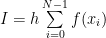
where 

Of course, you can try to do better. One could go into even more complex ones, but this section is only for introduction and comparisons.
The important thing to notice is that the methods accuracy is 

Monte Carlo Integration
A method of numerically calculating the integral is to use a random uniform distribution of points over the interval instead of equally spaced points (by the way, there are adaptive numerical methods that do not keep the h interval constant). It is quite obvious – using the Law of Large Numbers – that for a large number of samples the sum will approximate the integral.
Using the variance the error is estimated as 
Its power comes in the high dimensional spaces one meets very often. For example, in quantum mechanics the Hilbert space increases exponentially as one adds particles to the problem. Even in classical statistical physics, the dimensionality of the phase space is huge. Monte Carlo integration error is not exponentially dependent on the dimension of space like other methods and there is its strength!
Importance Sampling
There is a problem with the above Monte Carlo integration, the error depends on variance, too. It might be the case that you want to integrate a function that has significant value only in a small region (or in several). Using a uniform distribution will sample a lot of small values and might even miss the places where the function value is significant. Typically the number of possible state is huge and the number of samples that are taken into account in the Monte Carlo sum is very small compared with the number of possible states so it is very easy to miss the important ones. There are several ways of improving the method, here I’ll present briefly only one, the importance sampling.
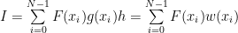
What can be done about it? Rewrite the integral:

If you use a function g that is approximately like f (ideally proportional with f, the proportionality being a constant) you get everywhere significant values – ideally F is everywhere constant. g(x) acts like a weight. Since g will be used as a probability distribution, it’s also required that:

To solve it with the computer, you transform it into a sum:
To be noted here that this method works for sums with many terms, too, not only for integrals. Also this is useful even for non Monte Carlo integration methods, just attempt to use a variable step size w instead of h and that is done for example in the adaptive methods.
The sum above for the Monte Carlo method is still for uniform random number distribution, but if one uses g(x) to generate the distribution instead of the uniform one, taking into account the Law of Large Numbers and the expected value one can see that the integral is approximated better. Now the function is sampled more in the regions where it has large values, the regions where it has low values being sampled less.
Markov chains
A Markov process is a process where evolution from the current state into the next one is dependent only on the current state, that is, it doesn’t depend on how the system got there (its history). For example, the usual random walk is a Markov chain, but the self avoiding random walk is not, because the possible next step depends on the system history.
Since I mentioned random walks, here is one implemented in JavaScript:
It starts in the center and restarts after the ‘particle’ reaches the boundary. Here is the source code:
1 2 3 4 5 6 7 8 9 10 11 12 13 14 15 16 17 18 19 20 21 22 23 24 25 26 27 28 29 30 31 32 33 34 35 36 | (function() { var canvas = document.getElementById("randomWalkCanvas"); var ctx = canvas.getContext("2d"); ctx.strokeStyle = "#000088"; var dist = canvas.height / 2.; ctx.translate(dist, dist); var posX = 0; var posY = 0; function randomWalk() { var dir = Math.floor(Math.random()*2); var sense = Math.floor(Math.random()*2); ctx.beginPath(); ctx.moveTo(posX,posY); if (dir == 0) posX += (sense ? 1 : -1)*4; else posY += (sense ? 1 : -1)*4; ctx.lineTo(posX,posY); ctx.stroke(); if (Math.abs(posX) > dist || Math.abs(posY) > dist) { posX = 0; posY = 0; ctx.clearRect(-dist, -dist, canvas.width, canvas.height); } } setInterval(randomWalk, 50); })(); |
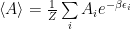
Now let’s particularize a little. We would like a Markov chain that samples the states in such a way that it helps us solve the integral (or sum) by importance sampling, that is, the chain should transition from one state to another with the probability needed for solving the sum, sampling the states the same way as the g distribution. To particularize further, in statistical physics the distribution that is often needed is:

where 


Very shortly, to obtain a way of getting the required distribution, one writes the master equation for the probability of being in a particular state and then he requires that the probability of being in a particular state is constant. This way one finds out that the probability of transitioning into a particular state during a period of time must be equal with the probability of transitioning out during the same period of time, that is, a balance equation. A particular solution that satisfies the equality is the detailed balance:

a, b are two particular states, p is the probability if being in a particular state and w gives the transition rate between them. Arranging the solution a little one finds:

This means that one can obtain a desired probability distribution just by having the proper transition probability between states in a Markov chain! The transition probability is then split in two, a choice probability and an acceptance ratio, 
Before finishing this section, I want to stress the ergodicity (see also this page) of the Markov chain. We want the process to sample the state space correctly, we don’t want it to end in a loop or to not be able to reach the relevant states.
Metropolis Algorithm
There are many methods that are using a Markov chain for Monte Carlo simulations, I want to mention for now here only one, the Metropolis-Hastings method, more precisely, the Metropolis algorithm which is a special case where the choice probability is symmetric, that is, the choice probability of picking b if the current state is a is equal with the one of picking a from the state b, 

There are many ways to choose the acceptance to obtain the desired ratio of probabilities, the Metropolis one is:
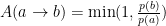
That is, if the probability of the state b is higher than the probability of state a, the state is always accepted, if not, the state b is accepted according to the ratio of probabilities. Even if ignoring all the previous discussion it is quite obvious how this favors high probability states but also samples the low probability ones.
The Monte Carlo Simulation
Let’s consider a case that is expected to be met in many statistical physics calculations, a Boltzmann distribution. For this case the ratio of probabilities turns into:

Very shortly, here is the algorithm, I’ll detail it when presenting an actual implementation:
- Pick a state at random. Sometimes it’s not that random, the algorithm might start with a state corresponding to an infinite or zero temperature.
- ‘Thermalize’ by walking along the Markov chain. Since the initial state might be quite far from the states that need to be sampled, the algorithm should be run for a while to allow reaching that region of the state space. The ‘walking’ is detailed below, it is similar with what happens after warmup.
- Pick the next state according with the choice probability.
- If the energy of the next state is lower than the energy of the current state, accept the new state., if not, accept it with the probability
.
- Continue with step 3 until enough states were generated. What’s ‘enough’ depends on the particular distribution and autocorrelation ‘time’ of the Markov chain.
- Use the current state for doing statistics and then go back to step 3.
Some brief implementation details: In many cases you don’t have to calculate again and again the energy or other values. Just notice that going from one state to another means an easily calculated change (often that’s the case) and use the difference to update the value. Also calculating some values involve exponentials. In many cases (for example when choosing a ‘next state’ involves some spin flip) the number of exponential values needed is limited. In such case it’s better to calculate them in advance and put them in a table to be reused, calculation of the exponentials all over again might be expensive.
Conclusions
I presented very briefly some things on the Monte Carlo methods, I’ll detail them further when presenting actual implementations.
Hopefully I’ll have more than one for this blog.
As usual, if you notice any mistakes, please let me know.
- Computational Physics A book by Konstantinos Anagnostopoulos ↩ ↩

The above mentioned book is also available using C++
Thank you!
The links are:
http://www.physics.ntua.gr/~konstant/ComputationalPhysics/
http://knanagnostopoulos.blogspot.com/2016/12/computational-physics-free-ebook.html